Knowledge Base / Glossary
Best-rank
The minimum vocabulary rank a pre-specified probe token hits across layers, positions, and allowed variants.
Best-rank is the smallest numerical vocabulary rank reached by a pre-specified probe across a search grid, typically layers × prompt positions × allowed token variants. Lower is stronger.
If \(r_{\ell,p,t}\) is the rank at layer \(\ell\), position \(p\), and token variant \(t\), then
\[ r_{\text{best}} = \min_{\ell,p,t} r_{\ell,p,t}. \]Although \(r_{\text{best}}\) is a minimum of numerical ranks, it is equivalent to maximizing a monotone evidence score such as \(-r\). It is therefore a best-of-many selection statistic; call it a max-statistic only when that transformed evidence score has been defined.
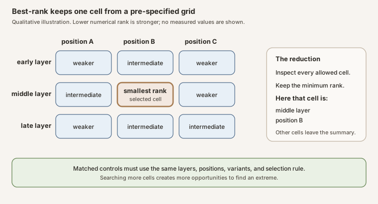
Scroll horizontally to inspect the diagram. The caption below provides a full text explanation.
Tiny implementation
def best_rank(ranks_by_layer_position):
    """Each cell contains ranks for the allowed token variants."""
    return min(
        rank
        for layer in ranks_by_layer_position
        for position in layer
        for rank in position
    )
The set of layers, positions, probes, and token variants must be fixed before comparing arms. Searching extra variants only for the favored condition makes the statistic incomparable.
Why matched controls matter
In an intentionally unrealistic null where \(N\) searched ranks are independent draws from the discrete uniform distribution on \(\{1,\ldots,V\}\), the exact expectation is
\[ \mathbb{E}[r_{\min}] = \sum_{j=1}^{V}\left(\frac{j}{V}\right)^N \approx \frac{V}{N+1}+\frac{1}{2}. \]With \(V=248{,}320\) and \(N=16{,}000\), the exact expectation is about 16.02; the approximation including the discrete continuity correction is also about 16.02. The cruder continuous approximation \(V/(N+1)\) is 15.52. Any of these is an impressive-looking rank generated by search alone. Real layer/position ranks are strongly dependent, so this is an intuition pump, not a null model for the experiment.
For each readout or transport, the Jacobian lens, the logit lens, and every random-J draw, apply the identical minimum separately to each pressure prompt and its matched control. Then compute paired pressure-control contrasts within each readout rather than treating the selected layer-position cell as an independent observation.
See also: rank, logit lens, prompt echo.