Late Chunking: Why Context-Aware Embeddings (sometimes) Beat Traditional Chunking

Problem: Lost Context in Embedding-Based Retrieval

In traditional RAG pipelines, we chunk documents before embedding. This breaks context by isolating sentences from their broader meaning. Consider this sample text about Berlin:

When you chunk by sentence and embed separately, contextual relationships are lost. Traditional chunking sees each sentence in isolation and can’t properly understand how terms relate across the full document context.

Analysis: Implementation and Results

Let’s build a systematic evaluation to test late chunking vs traditional chunking across different search scenarios. Here’s how we’ll implement and validate the approach:

Step 1: Setup and Dependencies

pip install transformers torch numpy pandas requests matplotlib seaborn scipy

Step 2: Our Test Document

We’ll use this Berlin document as our test case (adapted from the official Jina AI late chunking blog post):

input_text = ("Berlin is the capital and largest city of Germany, both by area and by population. "
              "Its more than 3.85 million inhabitants make it the European Union's most populous city, "
              "as measured by population within city limits. The city is also one of the states of Germany, "
              "and is the third smallest state in the country in terms of area.")

Note: This example and our implementation methodology are based on Jina AI’s original work, using their official Colab notebook as a starting point, which is linked from their late chunking blog post.

Step 3: Strategic Term Categories

We test 60 carefully chosen terms across two clear categories:

• HIGH Relatedness (17 terms): Berlin, Germany, Brandenburg, German capital, European Union, population, city, etc.
• LOW Relatedness (43 terms): Dogs, pizza, mountains, programming, music, colors, abstract concepts, etc.

Step 4: Directional Performance Logic

The key insight: “improvement” depends on what we’re searching for:

def calculate_directional_improvement(late_sim, trad_sim, expected_relatedness):
    raw_improvement = late_sim - trad_sim
    
    if expected_relatedness == 'high':
        # For related terms: higher similarity = better
        return raw_improvement, raw_improvement > 0
    elif expected_relatedness == 'low':
        # For unrelated terms: lower similarity = better (flip the sign!)
        return -raw_improvement, raw_improvement < 0

Step 5: Core Implementation

Load the model and setup:

from transformers import AutoModel, AutoTokenizer
import numpy as np

# Load Jina embeddings model
tokenizer = AutoTokenizer.from_pretrained('jinaai/jina-embeddings-v2-base-en', trust_remote_code=True)
model = AutoModel.from_pretrained('jinaai/jina-embeddings-v2-base-en', trust_remote_code=True)

Traditional chunking (chunk first, then embed):

# Split into sentences and embed each separately
chunks = split_by_sentences(input_text, tokenizer)
traditional_embeddings = [model.encode(chunk) for chunk in chunks]

Late chunking (embed full document, then chunk):

# Embed entire document first
inputs = tokenizer(input_text, return_tensors='pt')
model_output = model(**inputs)

# Then pool token embeddings by sentence spans
late_embeddings = late_chunking(model_output, sentence_spans)

Step 6: The Actual Comparison Process

Here’s exactly what we’re comparing:

The Setup:

• 4 chunks from our Berlin document (one sentence each)
• 60 test terms (Berlin-related vs completely unrelated)
• Two embedding methods for each chunk

What we calculate for each test term:

# For each test term (e.g., "Germany", "pizza", "population")
term_embedding = model.encode(term)

# For each of the 4 chunks, we get TWO similarity scores:
for chunk_idx, chunk_text in enumerate(chunks):
    
    # Method 1: Traditional chunking similarity
    traditional_chunk_embedding = model.encode(chunk_text)  # Embed chunk in isolation
    traditional_similarity = cosine_similarity(term_embedding, traditional_chunk_embedding)
    
    # Method 2: Late chunking similarity  
    late_chunk_embedding = late_embeddings[chunk_idx]  # From full-document context
    late_similarity = cosine_similarity(term_embedding, late_chunk_embedding)
    
    # Compare the two methods
    raw_improvement = late_similarity - traditional_similarity

Key Point: We’re comparing how well each method embeds the same chunk text, not comparing different chunks. Each chunk gets embedded two ways:

1. Traditional: Chunk embedded in isolation ("Berlin is the capital..." by itself)
2. Late: Same chunk but with full document context ("Berlin is the capital..." knowing about all 4 sentences)

Then we aggregate: For each term, we average across all 4 chunks to get overall performance for that term.

📁 Complete Implementation: demo.py

Note: Our implementation uses the official Jina AI late chunking Colab notebook as a starting point, extending it with related/unrelated terms, statistical analysis and visualization.

Key Insights from Visualization Analysis

1. Related vs Unrelated Comparison

This side-by-side comparison shows the core insight:

• Left panel (HIGH relatedness): Late chunking should produce higher bars (better similarity scores)
• Right panel (LOW relatedness): Late chunking should produce lower bars (prevents false matches)

The visualization clearly demonstrates late chunking’s context-awareness - it appropriately increases similarity for related terms while reducing false similarities for unrelated terms.

2. Performance Scatter Plot by Term Relatedness

This scatter plot reveals performance patterns across term types:

• RED points (high relatedness): Above diagonal = Late chunking wins
• BLUE points (low relatedness): Below diagonal = Late chunking wins (by giving lower scores)

Key observations:

• High-relatedness terms like “Berlin” and “Germany” show clear improvement with late chunking
• Low-relatedness terms demonstrate late chunking’s ability to avoid false matches

3. Directional Win Rates by Relatedness

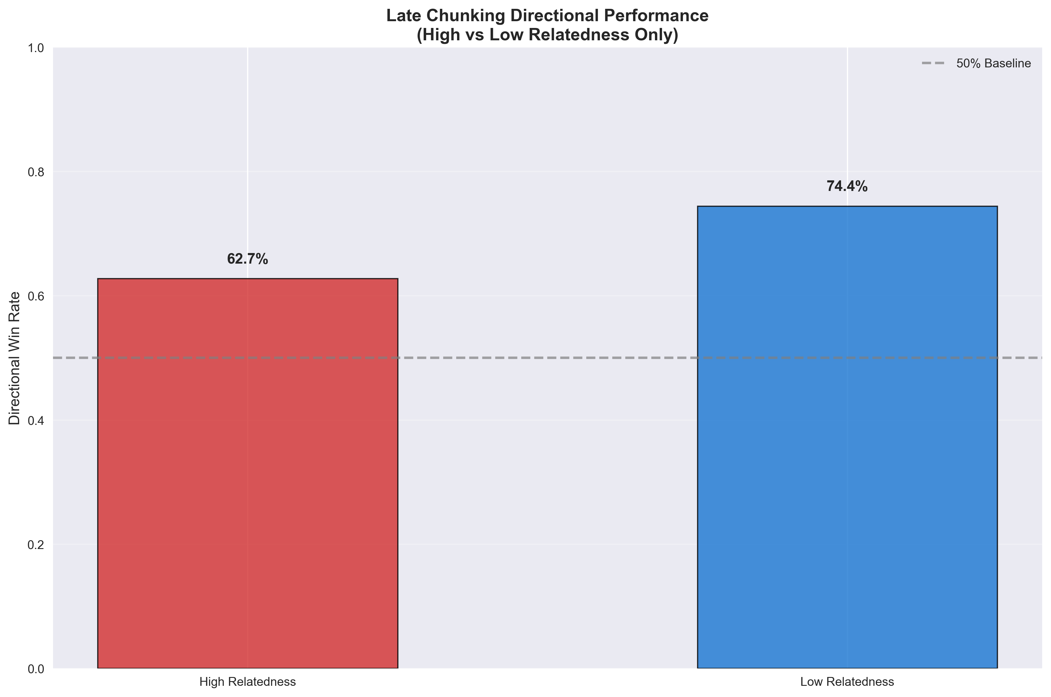
This chart shows late chunking’s context-aware performance:

• High Relatedness: 62.7% directional win rate (successfully finds relevant content)
• Low Relatedness: 74.4% directional win rate (successfully avoids false matches)

4. Improvement Distribution Analysis

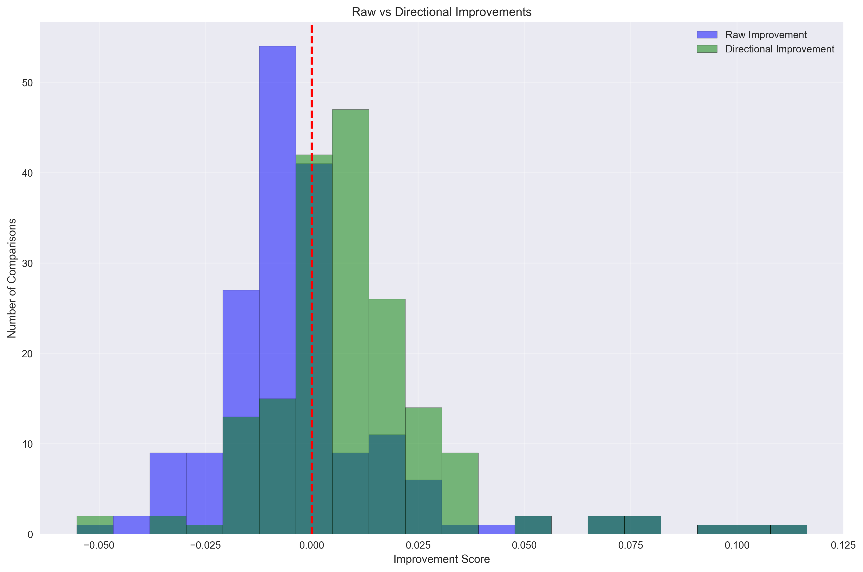
This histogram compares:

• Blue bars: Raw improvement (naive “higher = better” metric)
• Green bars: Directional improvement (context-aware metric)

The directional improvement distribution shows more positive values, indicating late chunking makes contextually appropriate decisions more often than raw metrics suggest.

5. Similarity Heatmaps by Term Relatedness

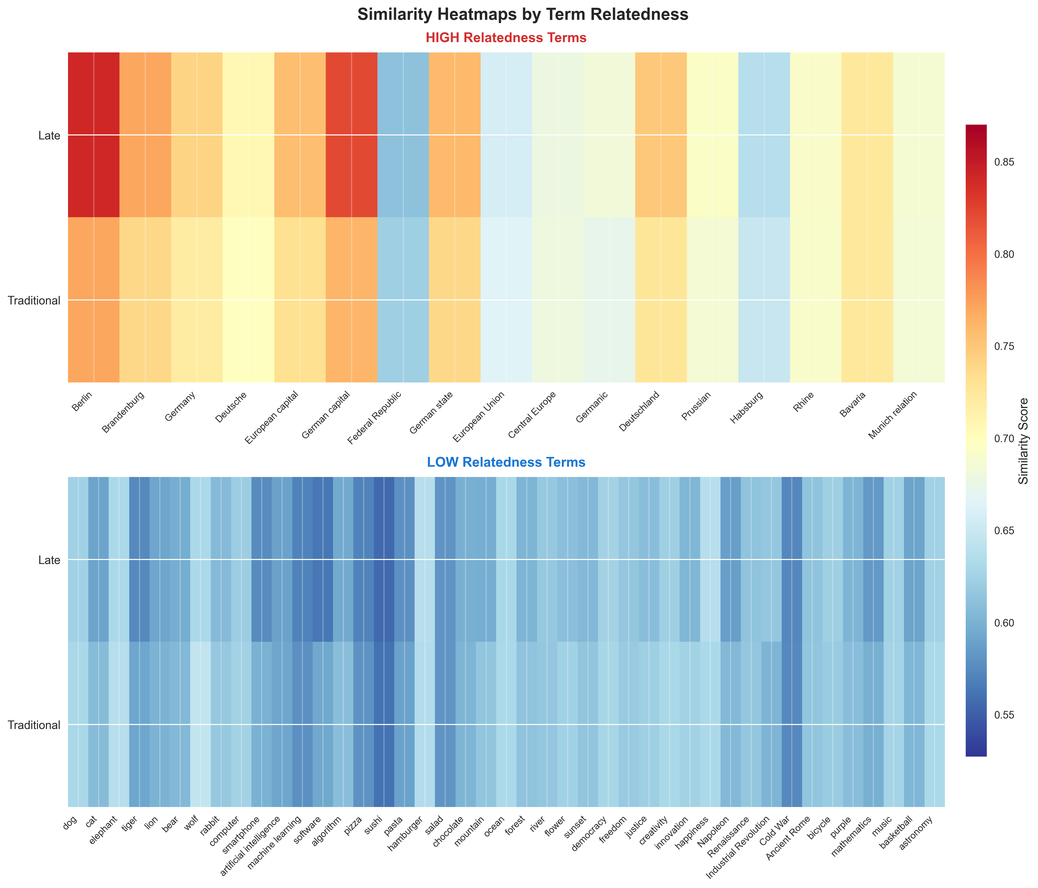
The stacked heatmaps reveal:

• HIGH Relatedness section: Should show red colors (high similarity) for good performance
• LOW Relatedness section: Should show blue colors (low similarity) for good performance

This visualization makes it immediately clear whether late chunking produces appropriate similarity scores for each term category.

Statistical Validation

Our analysis includes rigorous statistical testing to validate the significance of late chunking’s improvements:

Directional Improvements One-sample t-test

t-statistic: 4.2446
p-value: 0.000089
Significant: Yes (α = 0.05)

What this means:

• Null Hypothesis (H₀): Late chunking shows no directional improvement (mean = 0)
• Alternative Hypothesis (H₁): Late chunking shows positive directional improvement (mean > 0)
• t-statistic = 4.2446: A large positive value indicating strong effect
• p-value = 0.000089: Extremely small (< 0.001), much lower than 0.05 significance threshold

Interpretation: We can be 99.99%+ confident that late chunking’s directional improvements are real and not due to random variation within this specific experimental setup. The improvement is statistically significant for our test conditions.

Statistical Significance Explained

Important Statistical Limitations

Solution: Late Chunking Implementation

Late chunking fundamentally flips the traditional pipeline by reversing when we chunk and when we embed:

Key Advantages

Contextual Inheritance: Think of it like each sentence getting to “see” the entire document before deciding what it means. When the model processes “This method returns a cleaned DataFrame,” it already knows about the DataProcessor class and its process method from earlier in the document—so it creates a much richer, more informed representation.

Attention Across Boundaries: The Transformer’s self-attention mechanism can relate tokens across what would traditionally be separate chunks, creating richer representations that capture long-range dependencies.

Semantic Coherence: By embedding the full document first, we preserve the semantic relationships that span multiple sentences, reducing the fragmentation that occurs with traditional chunking.

Handling Large Documents

Yes, this is a significant practical limitation. Most transformer models have strict context limits (BERT: 512 tokens, many modern models: 2048-8192 tokens). When documents exceed these limits, you have several strategies:

1. Hierarchical Late Chunking

Split the document into context-sized sections first, then apply late chunking within each section:

def hierarchical_late_chunk(long_doc, max_tokens=512):
    # First-level chunking: split into model-sized chunks
    sections = split_by_token_limit(long_doc, max_tokens)
    
    # Second-level: late chunk within each section
    all_embeddings = []
    for section in sections:
        section_embeddings = late_chunk_section(section)
        all_embeddings.extend(section_embeddings)
    
    return all_embeddings

2. Sliding Window Approach

Process overlapping windows of the document to maintain some cross-boundary context:

def sliding_window_late_chunk(doc, window_size=400, overlap=50):
    windows = create_overlapping_windows(doc, window_size, overlap)
    return [late_chunk_window(window) for window in windows]

3. Hybrid Strategy

Use traditional chunking for very long documents, but late chunking for shorter ones:

def adaptive_chunking(doc, token_threshold=500):
    token_count = count_tokens(doc)
    if token_count <= token_threshold:
        return late_chunk(doc)  # Full late chunking
    else:
        return traditional_chunk(doc)  # Fall back to traditional

4. Modern Long-Context Models

Consider using models with extended context windows:

• Longformer: Up to 4,096 tokens
• LED (Longformer Encoder-Decoder): Up to 16,384 tokens
• GPT-4 Turbo: Up to 128,000 tokens
• Claude-3: Up to 200,000 tokens

Bottom Line: Late chunking works best for documents that fit comfortably within your model’s context window. For longer documents, you’ll need hybrid approaches that balance context preservation with practical constraints.

Frequently Asked Questions

Document-Specific Vector Relationships

Model Compatibility

Comparison with Advanced RAG Techniques

Handling Long Documents

Real-Time Application Considerations

Performance Interpretation

References

Core Late Chunking Research:

• Günther, M., & Xiao, H. (2024). Late Chunking in Long-Context Embedding Models. Jina AI. Link. The official Jina AI blog post introducing late chunking methodology with qualitative and quantitative evaluation on BEIR benchmarks.
• Günther, M., Mohr, I., Williams, D. J., Wang, B., & Xiao, H. (2024). Late Chunking: Contextual Chunk Embeddings Using Long-Context Embedding Models. arXiv. Link. The foundational academic paper with comprehensive evaluation demonstrating how chunking applied after transformer processing preserves full contextual information.
• Singh, B. (2024). Late Chunking: Embedding First Chunk Later — Long-Context Retrieval in RAG Applications. Stackademic. Link. Practical implementation guide detailing how late chunking embeds entire documents first to ensure every token’s embedding contains full context.

Advanced RAG Techniques:

• Govindaraj, P. (2024). Advanced RAG: Building and Evaluating a Sentence Window Retriever Setup Using LlamaIndex and Trulens. Medium. Link. Explores sentence window retrieval methods that preserve surrounding context.

Model and Architecture:

• Jina AI. (2023). Jina Embeddings V2: The First 8K Open-Source Text Embedding Model that Rivals OpenAI. Jina AI Blog. Link. Technical specifications for the embedding model used in our analysis, supporting up to 8192 tokens.
• Beltagy, I., Peters, M. E., & Cohan, A. (2020). Longformer: The Long-Document Transformer. arXiv. Link. Foundational work on long-context transformers using windowed attention mechanisms.

Vector Search Technology:

• Malkov, Y. A., & Yashunin, D. A. (2016). Efficient and robust approximate nearest neighbor search using Hierarchical Navigable Small World graphs. arXiv. Link. The HNSW algorithm underlying modern vector database search performance.