Knowledge Base / Glossary
Lyapunov exponent
The long-run exponential rate at which an infinitesimally small perturbation of a trajectory grows or shrinks.
A Lyapunov exponent is the long-run exponential rate, per step, at which an infinitesimally small perturbation of a trajectory grows or shrinks. For a differentiable map \(x_{k+1}=F(x_k)\), a perturbation \(v_k\) small enough that the map is effectively linear across it evolves by the derivative, \(v_{k+1}=DF(x_k)\,v_k\), where \(DF(x_k)\) is the Jacobian matrix of \(F\) at \(x_k\). Such a perturbation is called a tangent vector. After \(n\) steps, the finite-time rate is
\[ \lambda_n=\frac{1}{n}\ln\frac{\lVert v_n\rVert}{\lVert v_0\rVert}, \]where \(\lVert\cdot\rVert\) is the length of a vector and \(\ln\) is the natural logarithm, so the rate is measured in nats per step. The Lyapunov exponent is the limit of \(\lambda_n\) as \(n\) grows, when that limit exists. Oseledets’ theorem gives conditions under which it does, for almost every starting state with respect to an invariant measure, a fixed description of how often the trajectory visits each region of states. For a system in continuous time, elapsed time replaces the number of steps.
Two trajectories that start a finite distance apart follow this law only while their gap stays small. In a bounded system the gap eventually stops growing, and the ratio of distances at a late step then says nothing about the rate. Numerical estimates therefore follow a twin a small fixed distance from the reference, push it back to that distance after every step, and average the logarithms of the stretch factors. That is Benettin’s method, the one used in the note on chaos in a language model’s feedback loop.
A map of a \(d\)-dimensional state has \(d\) Lyapunov exponents, counted with multiplicity, each tied to a family of tangent directions; a perturbation in a generic direction grows at the largest one. A positive largest exponent means that infinitesimally close states separate exponentially, and it is the usual evidence of chaos, the one used for the soft-token loop. If the largest exponent is negative, every small perturbation along that trajectory dies out, as when the loop settles onto a stable fixed point or cycle. That is a statement about states near the trajectory, not about every starting state. A zero exponent marks a neutral direction, or growth slower than exponential.
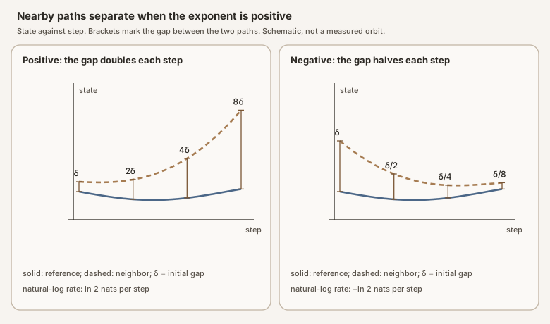
Scroll horizontally to inspect the diagram. The caption below provides a full text explanation.
Worked example
Suppose the length of a tangent vector exactly doubles every step and starts at \(10^{-3}\). After \(n\) steps it is \(10^{-3}\cdot 2^{n}\), and
\[ \lambda_n=\frac{1}{n}\ln(2^{n})=\ln 2\approx 0.693 \]for every \(n\). The starting length cancels. If instead the length were halved every step, the same calculation would give \(-\ln 2\).
from math import isfinite, log


def finite_time_exponent(initial_norm, final_norm, steps):
    """Log growth per step of one tangent vector evolved by the derivative."""
    if not isinstance(steps, int) or isinstance(steps, bool) or steps <= 0:
        raise ValueError("steps must be a positive integer")
    if not isfinite(initial_norm) or initial_norm <= 0:
        raise ValueError("initial_norm must be finite and positive")
    if not isfinite(final_norm) or final_norm < 0:
        raise ValueError("final_norm must be finite and nonnegative")
    if final_norm == 0:
        return float("-inf")
    return (log(final_norm) - log(initial_norm)) / steps
finite_time_exponent(1e-3, 1e-3 * 2**10, 10) returns \(\ln 2\). The helper evaluates the displayed formula from the lengths of a tangent vector; it does not evolve two trajectories or push a twin back after every step, as long numerical estimates do.
A positive finite-time estimate does not prove that the infinite-horizon exponent is positive, so a numerical report should state how many steps it measured, how many it discarded first as a transient, and how it followed the perturbation. The note’s chaos labels, for example, come from a twin at relative distance \(10^{-6}\), pushed back after every step, over 300 measured steps after 300 transient ones, with checks at 2000 measured steps after 1000 transient ones. The exponent is also not a next-token probability and not a measure of how often a particular word appears.
See also: Oseledets’ theorem, nat, Brouwer’s fixed-point theorem.