Knowledge Base / Glossary
Oseledets' theorem
If a differentiable map preserves a probability measure and its derivative is not too large on average, Lyapunov exponents exist at almost every state.
Oseledets’ multiplicative ergodic theorem gives the setting in which Lyapunov exponents exist as limits, not only as finite-run averages.
An invariant probability measure \(\mu\) is a distribution on states that the map leaves unchanged: pushing the distribution forward one step returns the same distribution. A continuous map of a nonempty compact set into itself always has at least one. That existence alone does not give the theorem, which also needs a derivative and a bound on its size.
Precisely, let \(F\) be a differentiable map of a \(d\)-dimensional state space that preserves a probability measure \(\mu\). Write \(\lVert DF(x)\rVert\) for the largest factor by which the derivative at \(x\) stretches a vector, and \(\ln^{+}r=\max(\ln r, 0)\). If \(\ln^{+}\lVert DF(x)\rVert\) has a finite average under \(\mu\), then for \(\mu\)-almost every state \(x\) and every nonzero tangent vector \(v\), the growth rate
\[ \lim_{n\to\infty}\frac{1}{n}\ln\big\lVert DF^n(x)\,v\big\rVert \]exists. It takes at most \(d\) different values, the Lyapunov exponents at \(x\), each belonging to a family of directions. A rate can be \(-\infty\) where the derivative is singular. Almost every means that the exceptional states form a set to which \(\mu\) assigns probability zero. The theorem holds more generally for products of matrices \(A(F^{n-1}x)\cdots A(x)\) along an orbit, called a linear cocycle, under the same condition on \(\ln^{+}\lVert A(x)\rVert\); the chain rule makes \(DF^n(x)\) such a product, with \(A=DF\).
An exponent computed from a finite run is a finite-time numerical estimate, not the infinite-horizon limit the theorem is about. The exponents reported in the note on chaos in a language model’s feedback loop are such estimates, from runs of 300 to 2000 measured steps.
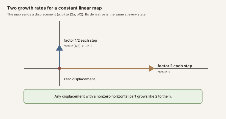
Scroll horizontally to inspect the diagram. The caption below provides a full text explanation.
Worked example
Let \(F(u,v)=(2u, v/2)\). Its derivative is the same matrix at every state:
\[ DF=\begin{bmatrix} 2 & 0 \\ 0 & \tfrac12 \end{bmatrix}, \qquad DF^n\begin{bmatrix} a \\ b \end{bmatrix}=\begin{bmatrix} 2^n a \\ 2^{-n} b \end{bmatrix}. \]If \(a\neq 0\), the length of the displacement grows like \(2^n\), and its rate is
\[ \frac{1}{n}\ln(2^n)=\ln 2\approx 0.693 \]per step. If \(a=0\) and \(b\neq 0\), the rate is \(\ln(1/2)=-\ln 2\). The two axes are the two exponent directions, at every state.
This map has no exceptional states to show, because the derivative never changes. The logistic map \(x\mapsto 4x(1-x)\) on \([0,1]\) has some. It preserves the probability density \(1/(\pi\sqrt{x(1-x)})\), under which almost every state has the exponent \(\ln 2\). The fixed point \(0\) has the exponent \(\ln 4\) instead, because the derivative there is 4. It is one of the exceptional states, and as a single point it has probability zero.
The theorem does not say that a short run has already reached these limits, or that a positive finite-time estimate is a proof of chaos.
See also: Lyapunov exponent, Brouwer’s fixed-point theorem.