Knowledge Base / Glossary
Monodromy
The derivative of one full trip around a periodic orbit: the ordered product of the step Jacobians.
The monodromy matrix of a periodic orbit is the derivative of one full trip around the cycle. If the orbit is \(x_1, x_2, \ldots, x_p\), with \(x_{k+1}=F(x_k)\) and \(x_{p+1}=x_1\), a tiny displacement at \(x_1\) is carried along by the Jacobian \(DF\) at each point. After one period the displacement has been multiplied by
\[ M = DF(x_p)\,DF(x_{p-1})\cdots DF(x_1). \]The last step’s Jacobian stands on the left, because it acts last. The eigenvalues of \(M\) are the orbit’s multipliers. They describe how one linearized trip around the cycle acts on small displacements: a real multiplier scales displacements along its eigenvector, and a pair of complex multipliers rotates and scales them within a plane. If every multiplier satisfies \(\lvert\mu\rvert<1\), the orbit is locally attracting: states close enough to it converge to it. If any multiplier has \(\lvert\mu\rvert>1\), the orbit is unstable, because some small displacements grow. When no multiplier lies outside the unit circle but some lie on it, \(\lvert\mu\rvert=1\), the linear part alone generally does not decide, and the nonlinear terms of the map do. In continuous-time Floquet theory, the analogous one-period evolution of the linearized equations is also called a monodromy matrix, and its eigenvalues are called Floquet multipliers.
One step can stretch while the cycle contracts. The monodromy is the product, so a large factor in a single Jacobian need not be a large multiplier.
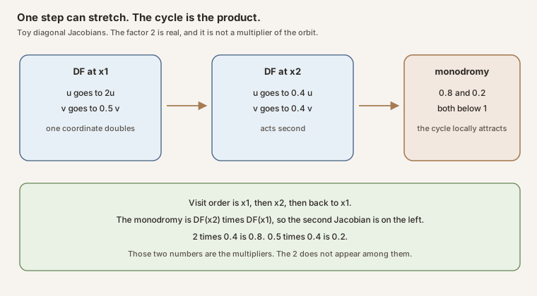
Scroll horizontally to inspect the diagram. The caption below provides a full text explanation.
Worked example
Let the two Jacobians be diagonal,
\[ DF(x_1)=\begin{bmatrix} 2 & 0 \\ 0 & 0.5 \end{bmatrix}, \qquad DF(x_2)=\begin{bmatrix} 0.4 & 0 \\ 0 & 0.4 \end{bmatrix}. \]The monodromy is
\[ M=DF(x_2)\,DF(x_1)=\begin{bmatrix} 0.8 & 0 \\ 0 & 0.2 \end{bmatrix}. \]A displacement \((u,v)\) at \(x_1\) returns as \((0.8u, 0.2v)\). The multipliers are \(0.8\) and \(0.2\). The factor \(2\) in the first Jacobian is real, and it is not a multiplier of the cycle.
def monodromy(jacobians):
    """Product DF(x_p) ... DF(x_1) of same-size square Jacobians listed in visit order."""
    if len(jacobians) == 0:
        raise ValueError("a cycle needs at least one Jacobian")
    width = len(jacobians[0])
    if width == 0 or any(
        len(jacobian) != width or any(len(row) != width for row in jacobian)
        for jacobian in jacobians
    ):
        raise ValueError("all Jacobians must be nonempty square matrices of the same size")
    product = [[1.0 if i == j else 0.0 for j in range(width)] for i in range(width)]
    for jacobian in jacobians:
        product = _matmul(jacobian, product)
    return product

def _matmul(left, right):
    width = len(left)
    return [
        [sum(left[i][k] * right[k][j] for k in range(width)) for j in range(width)]
        for i in range(width)
    ]
In this note the word is used for that cycle derivative, not for the monodromy of analytic continuation in complex analysis. A finite-precision product of many Jacobians can accumulate rounding error, and over long cycles it can overflow or underflow, even when each factor looks accurate. In the note on chaos in a language model’s feedback loop, a single float32 Jacobian-vector product along a period-8 orbit agrees with its float64 value to about \(5\times10^{-5}\), relatively. Yet the float32 8-step monodromy differs from the float64 one by about 3% in the Frobenius norm, the square root of the sum of squared entries, because the errors build up through a product of eight strongly contracting steps. That is why the note computes its orbits and multipliers in float64.
See also: Lyapunov exponent, Brouwer’s fixed-point theorem.