Knowledge Base / Glossary

Retrieval ranking metrics

Measures that compare a ranked retrieval list with relevance judgments, including position-discounted gain, recall, and reciprocal rank.

An information-retrieval system returns documents in an ordered list for a query. Retrieval ranking metrics summarize how that list agrees with relevance judgments, which are reference labels saying which documents count as relevant to that query. The notation @10 sets a cutoff: only ranks 1 through 10 are evaluated. Different metrics reward different things, so a report should name each metric rather than saying only that retrieval “improved.”

Three common metrics are:

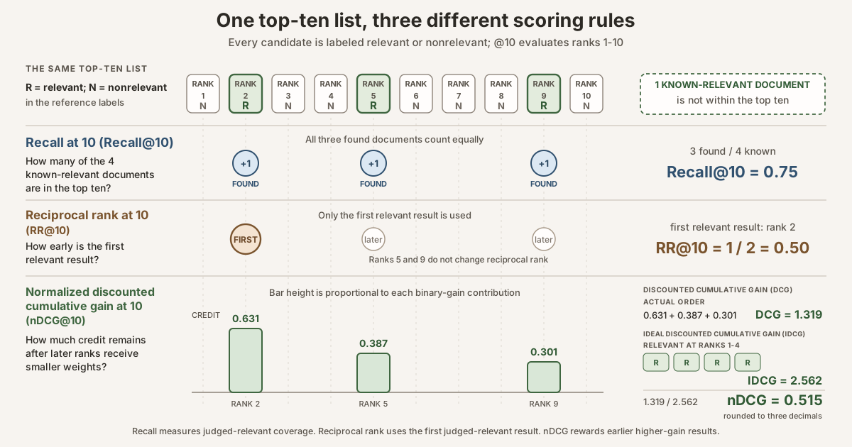
Recall@10 measures what fraction of the known relevant documents appear in the first 10 results;
reciprocal rank at 10 (RR@10) uses only the position of the first relevant result, giving 1 for rank 1, \(1/2\) for rank 2, and 0 when no relevant result appears by rank 10; and
normalized discounted cumulative gain at 10 (nDCG@10) rewards relevant documents near the top and can give more credit to highly relevant documents than partly relevant ones.

The reference labels are often stored as qrels, short for query relevance judgments. One query receives one RR@10 value. Mean reciprocal rank at 10 (MRR@10) is the arithmetic mean of those RR@10 values across a set of queries.

In a toy ranking, @10 means ranks 1 through 10 are evaluated and every candidate is labeled relevant or nonrelevant. Relevant documents occur at ranks 2, 5, and 9, while one of four known-relevant documents is not in the top ten. Recall counts all three found documents, reciprocal rank uses only rank 2, and normalized discounted cumulative gain gives the later results less credit. — Toy example with complete binary judgments, meaning every candidate document is labeled either relevant or nonrelevant; @10 means that only ranks 1 through 10 are evaluated. Four documents are known relevant; the top ten contains three at ranks 2, 5, and 9 and does not contain the fourth, so Recall@10 is 3/4 = 0.75. Reciprocal rank at 10 (RR@10) uses only the first relevant result, at rank 2, so RR@10 is 1/2 = 0.50; later relevant results do not affect RR. For normalized discounted cumulative gain at 10 (nDCG@10), the binary gains at ranks 2, 5, and 9 contribute 0.631, 0.387, and 0.301 to discounted cumulative gain at 10 (DCG@10) = 1.319. An ideal ordering places the four relevant documents at ranks 1 through 4 for ideal discounted cumulative gain at 10 (IDCG@10) = 2.562, giving nDCG@10 = 1.319 / 2.562 = 0.515 after rounding. The three scores answer different questions and are not interchangeable.

One ranked-list example

Suppose the reference labels identify four relevant documents for one query. The system places three of them at ranks 2, 5, and 9. The fourth does not appear within the top ten. It might appear below rank 10 or might not have been returned at all; this example does not need to decide which.

We will first use binary relevance: a relevant result has grade 1 and a nonrelevant result has grade 0. Later we will explain how nDCG can also use graded labels.

Recall@10

\[ \begin{aligned} \operatorname{Recall@10} &= \frac{\text{relevant documents found in the top 10}} {\text{known relevant documents}} \\ &= \frac{3}{4} = 0.75. \end{aligned} \]

The numerator is 3 because three known-relevant documents were found before the cutoff. The denominator is 4 because the reference labels contain four known-relevant documents in total. Recall ignores the order among the first 10 positions. Moving a relevant document from rank 9 to rank 2 would not change Recall@10.

Reciprocal rank and MRR@10

Let \(r\) be the rank of the first relevant result. For one query, reciprocal rank at 10 is

\[ \operatorname{RR@10} = \begin{cases} 1/r, & \text{if the first relevant result is at rank }r\le 10,\\ 0, & \text{if no relevant result appears by rank 10}. \end{cases} \]

The first relevant result in the example is at rank \(r=2\), so \(\operatorname{RR@10}=1/2=0.5\). Results at ranks 5 and 9 do not change that number. MRR@10 averages one such RR@10 value per query. It mostly answers “how soon did the first relevant result appear?” rather than “how many relevant results were found?”

nDCG@10

Let \(i\) identify a rank from 1 through 10, and let \(g_i\ge 0\) be the relevance grade of the document at that rank. With binary labels, \(g_i\) is either 0 or 1. With graded relevance, labels might instead use 0 for not relevant, 1 for partly relevant, and 2 for highly relevant. One common definition of discounted cumulative gain at 10 is

\[ \operatorname{DCG@10} = \sum_{i=1}^{10}\frac{2^{g_i}-1}{\log_2(i+1)}. \]

Read this as a sum of ten rank-by-rank contributions. The numerator \(2^{g_i}-1\) turns the relevance grade into a gain. Under binary relevance, a nonrelevant result contributes 0 and a relevant result contributes 1 before discounting. The denominator uses \(\log_2\), a base-two logarithm, to reduce the credit for later ranks. The \(i+1\) makes the rank-1 denominator \(\log_2(2)=1\) and avoids division by \(\log_2(1)=0\).

Only ranks 2, 5, and 9 contribute in the toy list:

\[ \begin{aligned} \operatorname{DCG@10} &= \frac{1}{\log_2(3)} + \frac{1}{\log_2(6)} + \frac{1}{\log_2(10)} \\ &\approx 0.631 + 0.387 + 0.301 = 1.319. \end{aligned} \]

That is the score for the returned ordering. To obtain ideal discounted cumulative gain at 10 (IDCG@10), rank all documents covered by the reference judgments, not just the returned top ten, from highest to lowest relevance grade and calculate DCG for the first 10 positions. In this complete-label toy example, the ideal ranking includes the fourth relevant document that was absent from the returned top ten and puts the four relevant documents at ranks 1 through 4:

\[ \operatorname{IDCG@10} = 1 + \frac{1}{\log_2(3)} + \frac{1}{\log_2(4)} + \frac{1}{\log_2(5)} \approx 2.562. \]

Finally, normalize the returned list’s DCG by that ideal value:

\[ \operatorname{nDCG@10} = \frac{\operatorname{DCG@10}}{\operatorname{IDCG@10}} = \frac{1.319}{2.562} \approx 0.515. \]

If a query has no known relevant documents, nDCG and recall need an explicit dataset or library convention rather than division by zero.

From per-query scores to a reported result

Evaluation commonly computes one score per query and then takes an unweighted mean across queries. This is macro-averaging: each query contributes equally even if queries have different numbers of relevant documents. Other aggregation choices are possible and should be named.

A query-level bootstrap repeatedly samples query units with replacement and recalculates the aggregate to summarize uncertainty. When comparing two systems, resample both systems’ scores for each selected query together so the pairing is preserved. An ordinary query bootstrap treats query units as exchangeable and approximately independent. Clustered or repeated queries need a blocked or cluster bootstrap that matches the study design. Any population interpretation is limited to the query population or sampling process represented by the evaluated query set.

What these metrics do not establish

A higher score does not prove that the retrieved text is factually correct or useful in a downstream biological decision.
Scores are conditional on the qrels, cutoff, query set, tie handling, and treatment of unjudged documents, meaning retrieved documents that have no label in the qrels.
MRR@10 does not reward a second relevant result, while Recall@10 does not reward earlier ordering within the top 10.
Differences between systems need paired per-query analysis; two rounded averages alone do not show how consistently one system wins.