Knowledge Base / Glossary
Log loss
The average negative logarithm of the probability a model gave to what actually happened, so confident mistakes cost far more than cautious ones.
A model states a probability that something will happen, then the outcome arrives. Log loss grades that forecast by asking one question of every case: what probability did you put on the thing that actually happened? Each case is charged the negative natural logarithm of that probability, and the charges are averaged. Saying 0.99 about something that happened costs almost nothing. Saying 0.001 about something that happened costs a great deal.
Log loss is also called cross-entropy loss, and in this two-outcome setting binary cross-entropy. For independent Bernoulli outcomes it is the negative log likelihood divided by the number of cases, so watch that convention: some software and some texts reserve that name for the unnormalized sum. Lower is better, the best possible value is 0, and there is no upper bound.
The definition
Take \(n\) cases. For case \(i\), let \(p_i\) be the stated probability of the positive outcome and let \(y_i\) be the outcome indicator: 1 if the positive outcome happened and 0 if it did not. Writing \(\log\) for the natural logarithm,
\[ \mathrm{log\ loss}=-\frac{1}{n}\sum_{i=1}^{n} \left[y_i\log(p_i)+(1-y_i)\log(1-p_i)\right]. \]Only one of the two bracketed terms is ever alive, because \(y_i\) is either 1 or 0. A positive case contributes \(-\log(p_i)\); a negative case contributes \(-\log(1-p_i)\). In both branches, \(p_i\) or \(1-p_i\) is the probability the model assigned to what actually happened, so the whole formula is the plain sentence at the top of this page written in symbols.
Reading the penalty
The natural logarithm of a probability is never positive, so the leading minus sign turns every charge into a nonnegative cost. The cost is 0 at perfect confidence in the truth, rises gently through the middle of the range, and then climbs without limit.
| Probability the model gave to what actually happened | Row penalty \(-\log(\cdot)\) |
|---|---|
| 0.99 | 0.01 |
| 0.90 | 0.11 |
| 0.50 | 0.69 |
| 0.10 | 2.30 |
| 0.01 | 4.61 |
| 0.001 | 6.91 |
Each tenfold step toward zero adds another 2.30, forever. That is the whole character of the measure: it is close to indifferent between 0.90 and 0.99, and brutal about the difference between 0.01 and 0.001.
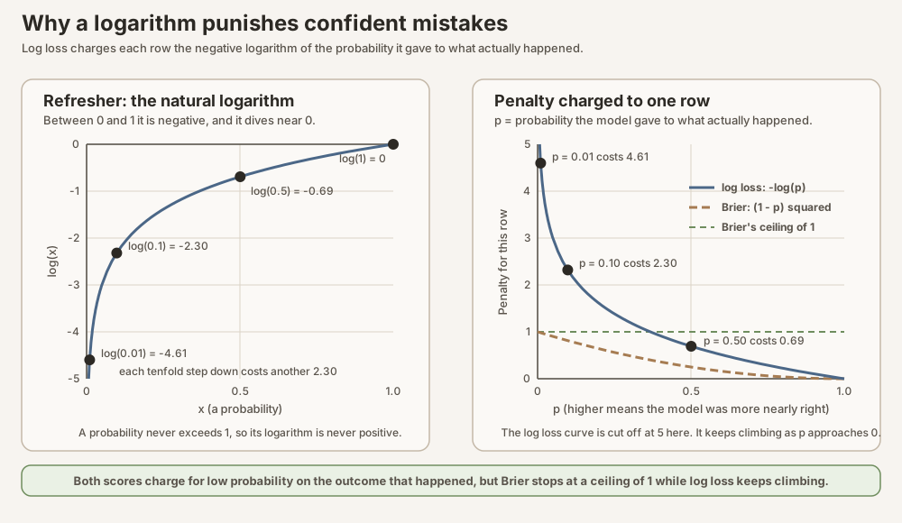
Scroll horizontally to inspect the diagram. The caption below provides a full text explanation.
A worked example you can check by hand
The same five cases used in the Brier loss entry, now charged the logarithmic way. The fourth column picks out the probability the model gave to what actually happened, which is \(p_i\) when the case was positive and \(1-p_i\) when it was negative.
| Case | Stated \(p_i\) | Outcome \(y_i\) | Probability on the truth | Penalty |
|---|---|---|---|---|
| 1 | 0.90 | 1 | 0.90 | 0.1054 |
| 2 | 0.80 | 1 | 0.80 | 0.2231 |
| 3 | 0.30 | 0 | 0.70 | 0.3567 |
| 4 | 0.10 | 0 | 0.90 | 0.1054 |
| 5 | 0.02 | 1 | 0.02 | 3.9120 |
The five penalties sum to 4.7026, so the log loss is \(4.7026/5=0.9405\). Case 5 alone supplies 83 percent of it. Restate that one forecast as a shrug at 0.50, leaving the other four untouched, and the log loss falls to 0.2967; leave it out entirely and the remaining four average 0.1976.
Compare that with Brier loss on the identical five rows: 0.2221 with case 5, and 0.0375 without it. Both measures agree that the confident miss was the story, and in this particular example both are dominated by it, case 5 supplying about 83 percent of the log loss total and about 86 percent of the Brier total. The difference between the two rules is not their verdict here but what happens as a forecast gets worse: a single Brier charge can never exceed 1, while a log loss charge grows without limit as the probability given to the truth approaches zero. Push case 5 from 0.02 down to 0.0002 and its Brier charge creeps from 0.9604 to 0.9996, while its log loss charge more than doubles, from 3.9120 to 8.5172.
Why the penalty has no ceiling
Squared error, the ingredient in Brier loss, tops out at 1 because probabilities and outcomes both live in \([0,1]\). The logarithm has no such limit: as the probability assigned to the truth goes to zero, \(-\log(p)\) goes to infinity. Stating probability 0 for something that then happens is, under this rule, an infinitely expensive claim, which is a defensible way to grade a forecaster who declared an actual event impossible.
It is also a practical hazard, since one such case would make the average
infinite regardless of how well everything else went. Many implementations
therefore clip predicted probabilities away from exactly 0 and 1 before taking
the logarithm; scikit-learn’s log_loss does this and documents the behavior in
its model-evaluation guide
(official guide).
Others do not, and return infinity or a not-a-number value at the boundary
unless the caller clips first, which is exactly what the bare NumPy expression
further down this page would do. Report the implementation, its version, and
its clipping convention when the extremes matter, because clipping silently
sets the worst price any single case can pay.
The no-skill anchor moves with the base rate
A forecaster that ignores every feature and repeats the overall positive rate \(\bar o\) on every case scores
\[ -\left[\bar o\log\bar o+(1-\bar o)\log(1-\bar o)\right], \]which is the entropy of the label distribution: a measure of how uncertain the outcome was before any model spoke. That is the number a real model has to beat, and it depends only on the labels. Reading \(\bar o\) off the very cases being scored makes this a hindsight anchor rather than a baseline anyone could have deployed; a constant forecast you could actually have shipped takes its rate from training or historical data and is then scored, unchanged, on the held-out cases.
The anchor is largest at \(\bar o=0.5\), where it equals \(\log 2=0.6931\), and it shrinks as the outcome becomes lopsided. In an illustrative set with 328 positives among 3,580 cases, \(\bar o=0.0916\) and the anchor is 0.3063. A log loss of 0.25 beats both of those anchors, but it means very different things against each: a huge improvement on the balanced problem and a slim one on the rare-positive problem, where simply repeating the base rate already scores 0.3063. Quote the anchor beside the score, or report the improvement over it, and do not compare raw log losses across datasets whose base rates differ. See base-rate bias for the wider version of that error.
Strict properness, or why truthful probabilities win on average
Log loss is a strictly proper scoring rule. A scoring rule is any recipe for grading a stated probability against what actually happened; a rule is proper when the lowest expected penalty comes from reporting the actual probability of the outcome, and strictly proper when that report is the only way to reach the lowest expected penalty (Gneiting and Raftery, 2007).
Concretely, take a group of cases that truly go positive 70 percent of the time, and suppose one number \(q\) has to be stated for every case in the group. Averaging over that 70/30 split of outcomes:
| Reported \(q\) | Expected log loss \(-[0.7\log q+0.3\log(1-q)]\) | Expected Brier loss \(0.7(1-q)^2+0.3q^2\) |
|---|---|---|
| 0.50, hedging to the middle | 0.6931 | 0.2500 |
| 0.60 | 0.6325 | 0.2200 |
| 0.70, the true rate | 0.6109 | 0.2100 |
| 0.90 | 0.7645 | 0.2500 |
| 0.99, sounding decisive | 1.3886 | 0.2941 |
Both columns bottom out at \(q=0.70\), the rate at which these cases actually turn out positive, which is what properness means. They disagree about how badly overconfidence should hurt: moving from 0.70 to 0.99 costs about 0.08 of expected Brier loss and about 0.78 of expected log loss, nearly ten times as much. “Expected” means averaged over those outcomes in the long run, so the guarantee is about that average and not about any single case, where luck can always make a well-stated probability look bad.
The rule was originally designed for human forecasters, which is why the older literature phrases it as an incentive to report your honest belief. For a fitted model the statement is simpler: its expected log loss is smallest, and uniquely so, when its output for a group of similar rows equals the rate at which such rows actually turn out positive, and no post-processing of the probabilities helps unless it moves them toward those rates.
The guarantee is about expected loss in the population, which is not the same as saying a reported number cannot be flattered. Overfitting, leakage, model selection against the evaluation labels, and repeated reuse of the same test set all still inflate how good an empirical log loss looks. Strict properness makes the score worth measuring; a genuinely held-out evaluation is what makes the measurement mean something.
Computing it
import numpy as np
from sklearn.metrics import log_loss

p = np.array([0.90, 0.80, 0.30, 0.10, 0.02])
y = np.array([1, 1, 0, 0, 1])

log_loss(y, p)                                       # 0.9405
-np.mean(y * np.log(p) + (1 - y) * np.log(1 - p))    # 0.9405, the same arithmetic
Three conventions worth stating whenever you report the number. First, the logarithm base: natural logarithms give the value above, while base-2 logarithms report the same quantity in bits and are 1.4427 times larger. Second, how probabilities map to classes: for a one-dimensional binary array, say which class that probability belongs to, and note that swapping the class roles consistently, using \(y'=1-y\) and \(p'=1-p\), leaves the score unchanged. The multiclass form sums \(-y_{ik}\log(p_{ik})\) over the classes within each case, where only the true class survives one-hot labels, and then averages over cases; state as well whether your implementation returns a sum or a mean and whether cases carry weights. Third, whether the score was computed on held-out cases; a log loss measured on the rows a model was fitted to is a training diagnostic, not evidence about future forecasts.
What a log loss does not establish
- It does not certify calibration. Read it beside a reliability diagram, which displays whether stated probabilities match observed rates bin by bin (Niculescu-Mizil and Caruana, 2005).
- It is not comparable across datasets with different base rates, because the no-skill anchor travels with the labels rather than the model.
- It is not a ranking metric. Two models can order cases identically and still post different log losses, since the rule grades the stated numbers.
- It says nothing about workload at a chosen threshold. Precision, recall, and the count of false alarms need a threshold; log loss never uses one.
- A single number can be dominated by a handful of confident misses. Inspect the largest per-case penalties before concluding that a model is broadly worse, and quantify the uncertainty in the paired per-case difference between the two models rather than in each score on its own. A bootstrap has to resample the same evaluation units for both models and preserve any grouping or time ordering in the data.
See also: Brier loss, base-rate bias, bootstrap, independent and identically distributed (i.i.d.), and the Deep Dive Logistic Regression and Random Forest, where both probability scores are reported on a fixed holdout.