Knowledge Base / Glossary
Brier loss
The average squared gap between a stated probability and the zero-or-one outcome that followed, so lower means better probability forecasts.
Suppose something either happens or it does not, and before it resolves a model states a probability that it will. A weather model says 0.30 for rain; a classifier says 0.90 that a candidate signal is a real pulsar. Once the outcome is known, how good was the number?
Brier loss answers that by charging each forecast the square of its distance from what actually happened, then averaging the charges. It is the mean squared error of probabilities. Zero is perfect, higher is worse, and the worst possible value is 1.
The definition
Take \(n\) cases. For case \(i\), let \(p_i\) be the stated probability of the positive outcome, a number between 0 and 1, and let \(y_i\) be the outcome indicator: 1 if the positive outcome happened and 0 if it did not. Then
\[ \mathrm{Brier}=\frac{1}{n}\sum_{i=1}^{n}(p_i-y_i)^2. \]Each row contributes \((p_i-y_i)^2\), the squared distance between the number stated and the number that turned out to be true. Because \(p_i\) and \(y_i\) both live in \([0,1]\), no single row can be charged more than 1, so the average cannot exceed 1 either.
Some writers call the same quantity the Brier score (Brier, 1950). Under the binary, one-probability convention used here, the two names refer to the identical formula and the value ranges from 0 to 1. State the convention when you report it, because another common formulation sums the squared errors over both class probabilities; in the two-class case that version is twice the formula above and ranges from 0 to 2. This site uses the one-probability formula and says Brier loss throughout so that “lower is better” is never ambiguous; if you meet “Brier score” in a caption or a receipt here, read it as the same mean squared error.
A worked example you can check by hand
Five candidates were scored, then their true labels arrived. The last row is the interesting one: the model was confident and wrong.
| Case | Stated \(p_i\) | Outcome \(y_i\) | \((p_i-y_i)^2\) |
|---|---|---|---|
| 1 | 0.90 | 1 | 0.0100 |
| 2 | 0.80 | 1 | 0.0400 |
| 3 | 0.30 | 0 | 0.0900 |
| 4 | 0.10 | 0 | 0.0100 |
| 5 | 0.02 | 1 | 0.9604 |
The five charges sum to 1.1104, so the Brier loss is \(1.1104/5=0.2221\). Drop case 5 and the remaining four average 0.0375. One confident mistake in five rows made the average nearly six times larger, but notice the ceiling: even a forecast of 0.00 on a case that happened would have been charged only 1.00. That bounded worst case is the main behavioral difference from log loss, which charges an unbounded penalty for the same mistake.
One number, three separate jobs
A Brier loss is not purely a measure of whether stated probabilities match observed frequencies. It also absorbs how hard the outcome was to predict at all, and how well the model separated cases from one another. Those three effects can be written out exactly.
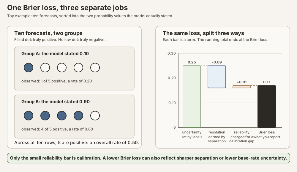
Scroll horizontally to inspect the diagram. The caption below provides a full text explanation.
Group the cases by the probability they were given, the same grouping a reliability diagram uses: a plot of each group’s observed positive rate against the probability that group was told, where perfect agreement on these rows puts every group on the diagonal. Say there are \(K\) groups; group \(k\) holds \(n_k\) cases that all received the same stated probability \(p_k\), and a fraction \(\bar o_k\) of them turned out positive. Let \(\bar o\) be the positive rate across all \(n\) cases. Then
\[ \mathrm{Brier} =\frac{1}{n}\sum_{k=1}^{K}n_k\left(p_k-\bar o_k\right)^2 -\frac{1}{n}\sum_{k=1}^{K}n_k\left(\bar o_k-\bar o\right)^2 +\bar o\left(1-\bar o\right). \]| Term | Usual name | What it asks | Direction |
|---|---|---|---|
| \(\frac{1}{n}\sum_k n_k(p_k-\bar o_k)^2\) | reliability | Inside one group, does the stated probability match the observed rate? | smaller is better; this term is calibration |
| \(\frac{1}{n}\sum_k n_k(\bar o_k-\bar o)^2\) | resolution | Do the groups the model creates have observed rates far from the overall rate? | larger is better, and it is subtracted |
| \(\bar o(1-\bar o)\) | uncertainty | How uncertain was the outcome before any model spoke? | fixed by the labels, not by the model |
This partition is due to Murphy (1973). It is the same quantity as the definition above, rewritten, not a second measurement. Split the rows into groups and expand each squared error inside group \(k\) around that group’s observed rate: the cross term drops out because deviations from a group mean sum to zero, and because \(y_i\) is 0 or 1 the leftover within-group spread is exactly \(n_k\bar o_k(1-\bar o_k)\). Summing that spread over groups and re-centering it on the overall rate turns it into \(\bar o(1-\bar o)-\frac{1}{n}\sum_k n_k(\bar o_k-\bar o)^2\), which is uncertainty minus resolution. No approximation enters anywhere: every term is computed from the rows in front of you, and the identity holds exactly for that sample. The group rates are still sample quantities, though, so a group that looks calibrated on these rows has not thereby been shown to be calibrated on future ones.
The same toy, both ways
Take the ten forecasts in the figure. Five were told 0.10 and one of them was positive; five were told 0.90 and four of them were positive.
Directly from the definition: the four charges in the first group are \((0.10-1)^2=0.81\) once and \((0.10-0)^2=0.01\) four times; the second group gives \((0.90-1)^2=0.01\) four times and \((0.90-0)^2=0.81\) once. The ten charges sum to 1.70, so the Brier loss is 0.17.
Through the partition, with \(\bar o=0.5\):
- reliability \(=\frac{1}{10}\left[5(0.10-0.20)^2+5(0.90-0.80)^2\right]=0.01\)
- resolution \(=\frac{1}{10}\left[5(0.20-0.50)^2+5(0.80-0.50)^2\right]=0.09\)
- uncertainty \(=0.5\times 0.5=0.25\)
and \(0.01-0.09+0.25=0.17\), the same number. Now make the model perfectly calibrated on these ten rows by restating those probabilities as 0.20 and 0.80, the rates its own groups actually showed. Reliability falls to 0, resolution and uncertainty do not move, and the Brier loss becomes 0.16. The calibration repair was worth exactly the 0.01 that reliability was charging.
The partition needs groups, and continuous forecasts fight it
The identity above is exact when every case in a group received the same stated probability. Real models rarely oblige. A fitted classifier emits effectively continuous probabilities, so strict grouping puts nearly every row in a group of its own, and in a group of one \(\bar o_k\) is simply that row’s label. Plug that degenerate grouping into the three terms and watch them stop being useful:
- reliability becomes \(\frac{1}{n}\sum_i(p_i-y_i)^2\), which is the whole Brier loss again;
- resolution becomes \(\frac{1}{n}\sum_i(y_i-\bar o)^2=\bar o(1-\bar o)\), which is exactly the uncertainty term.
Write the partition out with those substitutions:
\[ \mathrm{Brier} =\mathrm{Brier} -\bar o(1-\bar o) +\bar o(1-\bar o). \]That looks circular, but it is not a new transform. The three right-hand terms are still reliability, then minus resolution, then plus uncertainty; they just happen to evaluate to \(\mathrm{Brier}\), \(\bar o(1-\bar o)\), and \(\bar o(1-\bar o)\) in this degenerate grouping. The last two cancel, so the identity reduces to \(\mathrm{Brier}=\mathrm{Brier}\): algebraically true, diagnostically empty. Nothing has been separated, because the entire loss sits back inside the first term.
Reading the partition on real predictions therefore means grouping nearby probabilities into bins and putting each bin’s mean forecast \(\bar p_k\) where a single stated probability used to be. Once forecasts vary inside a bin, the three displayed terms no longer add up on their own. Restoring the exact identity takes a fourth term,
\[ R=\frac{1}{n}\sum_{k=1}^{K}\sum_{i\in k} \left[(p_i-\bar p_k)^2-2(p_i-\bar p_k)(y_i-\bar o_k)\right], \]which collects the spread of forecasts inside a bin and any agreement between that spread and the outcomes. It is not guaranteed to be small, and it can be negative. The total on the left never moves. The three named pieces and \(R\) do, and they shift when you change the bin edges, exactly as a reliability diagram does. Treat the binned partition as a way of reading the number, not as a rival measurement.
The no-skill anchor moves with the base rate
A forecaster that ignores every feature and repeats one constant \(q\) on every case has no resolution at all, and its Brier loss works out to \(\bar o(1-\bar o)+(q-\bar o)^2\). The best it can do is set \(q=\bar o\), the positive rate of the very cases being scored, which lands it exactly on the uncertainty term \(\bar o(1-\bar o)\). That is the anchor a real model has to beat, with one caveat worth keeping in view: choosing \(q\) from the evaluation labels is hindsight. A constant baseline you could actually have deployed takes its rate from training or historical data, so its held-out loss sits slightly above the held-out uncertainty term by the squared gap between the two rates.
The anchor depends only on how common the outcome is, and it is largest at \(\bar o=0.5\), where it equals 0.25. On a dataset where positives are rare it is small: in an illustrative set with 328 positives among 3,580 cases, \(\bar o=0.0916\) and the anchor is \(0.0916\times 0.9084=0.0832\). A model scoring 0.07 there sounds excellent next to a model scoring 0.20 on a balanced dataset, yet the second model may be doing far more work. Always quote the base-rate anchor beside the Brier loss, and never compare raw Brier losses across datasets whose positive rates differ. See base-rate bias for the more general version of that mistake.
Strict properness, or why truthful probabilities win on average
Brier loss is a strictly proper scoring rule. A scoring rule is any recipe for grading a stated probability against what actually happened; a rule is proper when the lowest expected charge comes from reporting the actual probability of the outcome, and strictly proper when that report is the only way to reach the lowest expected charge (Gneiting and Raftery, 2007).
Concretely, take a group of cases that truly go positive 70 percent of the time, and suppose you have to state one number \(q\) for every case in the group. Averaging over that 70/30 split of outcomes, your expected charge is \(0.7(1-q)^2+0.3q^2\):
| Reported \(q\) | Expected Brier loss |
|---|---|
| 0.50, hedging to the middle | 0.2500 |
| 0.60 | 0.2200 |
| 0.70, the true rate | 0.2100 |
| 0.90 | 0.2500 |
| 0.99, sounding decisive | 0.2941 |
The minimum sits at \(q=0.70\), the rate at which these cases actually turn out positive, and the charge rises in both directions away from it. “Expected” means averaged over those outcomes in the long run; the guarantee is about that average, not about any single case, where luck can always make a well-stated probability look bad.
The rule was originally designed for human forecasters, which is why the older literature phrases it as an incentive to report your honest belief. For a fitted model there is no belief to be honest about, and the statement becomes simpler: the model’s expected Brier loss is smallest, and uniquely so, when its output for a group of similar rows equals the rate at which such rows actually turn out positive. Nothing can be gained by post-processing the probabilities in any way that does not move them toward those rates.
That guarantee is about expected loss in the population, so it does not make a reported number unfalsifiable. Selecting a model on the evaluation labels, tuning against them, leaking them into features, or reusing the same test set many times can still make an empirical Brier loss look better than the model deserves. Properness earns you the right to read the number as a measurement of probability quality; a genuinely held-out evaluation is what earns you the number.
Computing it
import numpy as np
from sklearn.metrics import brier_score_loss

p = np.array([0.90, 0.80, 0.30, 0.10, 0.02])
y = np.array([1, 1, 0, 0, 1])

brier_score_loss(y, p)     # 0.22208
np.mean((p - y) ** 2)      # 0.22208, the same arithmetic
Two conventions to state when you report the number. First, which class the probability refers to: \(p\) has to be the probability of the class encoded as \(y=1\). Swap the roles consistently, using \(y'=1-y\) and \(p'=1-p\), and the binary Brier loss is unchanged; flip only the labels or only the probabilities and you have simply mismatched the inputs. Second, whether the score is computed on held-out cases; a Brier loss measured on the rows a model was fitted to is a training diagnostic, not evidence about future forecasts. scikit-learn’s model-evaluation guide documents its own conventions (official guide).
What a Brier loss does not establish
- It does not certify calibration. Only the reliability term is calibration, and a model can post a good Brier loss on strong separation while a middle bin sits well off the diagonal. Read it beside a reliability diagram (Niculescu-Mizil and Caruana, 2005).
- It is not comparable across datasets with different base rates, because the uncertainty term travels with the labels rather than the model.
- It says nothing directly about the review workload at a chosen threshold. A Brier loss is computed from probabilities and outcomes without ever applying a decision threshold; precision, recall, and the count of false alarms need one.
- It is not a ranking metric. Two models can share a ranking and differ in Brier loss, and two models can share a Brier loss and rank cases differently.
- A single held-out Brier loss is one draw. When two models were scored on the same cases, quantify the uncertainty in their paired per-case differences rather than in each score separately, and resample at whatever unit is actually independent, keeping any clustering or time ordering intact. A bootstrap over held-out rows describes uncertainty given the fitted models; covering training variability as well means refitting inside the resampling.
See also: log loss, Gini impurity, base-rate bias, bootstrap, independent and identically distributed (i.i.d.), and the Deep Dive Logistic Regression and Random Forest, where both scores are reported on a fixed holdout.