Next-token entropy

Next-token entropy is the Shannon entropy of the probabilities a language model assigns to the possible next tokens at one step. A token is one item in the model’s vocabulary, the fixed set of items it can process or produce, such as word pieces, punctuation marks, or bytes. Next-token entropy measures how spread out that prediction is. It does not name the winning token, and it is not a count of how many tokens have nonzero probability.

Let \(H\) denote the next-token entropy, let \(p_t\) be the probability of token \(t\) (with every \(p_t\ge 0\) and \(\sum_t p_t = 1\)), and let \(\ln\) denote the natural logarithm, whose base is \(e\approx 2.71828\). In nats, the natural-logarithm unit of information,

The sum runs over the vocabulary. The convention \(0\ln 0=0\) makes a token with probability zero contribute nothing. If one token has probability 1, then \(H=0\): the prediction is certain. If the probability is spread evenly over \(N\) tokens, then \(H=\ln N\). Reading an entropy backward, \(e^{H}\) is the number of tokens in an even choice with that same entropy. That count is an effective number of equally likely choices. A real distribution with the same \(H\) need not be even.

Language models produce logits, their unnormalized output scores. For standard temperature scaling with a positive temperature \(T > 0\), if \(z_t\) is token \(t\)’s logit, then

where the denominator sums over all vocabulary tokens \(j\). This normalization is the softmax function (\(T = 1\) gives ordinary softmax, while \(T = 0\) is not inserted into this division). If the probabilities are modified again by another rule, \(H\) refers to whichever normalized probability distribution is supplied to the entropy formula.

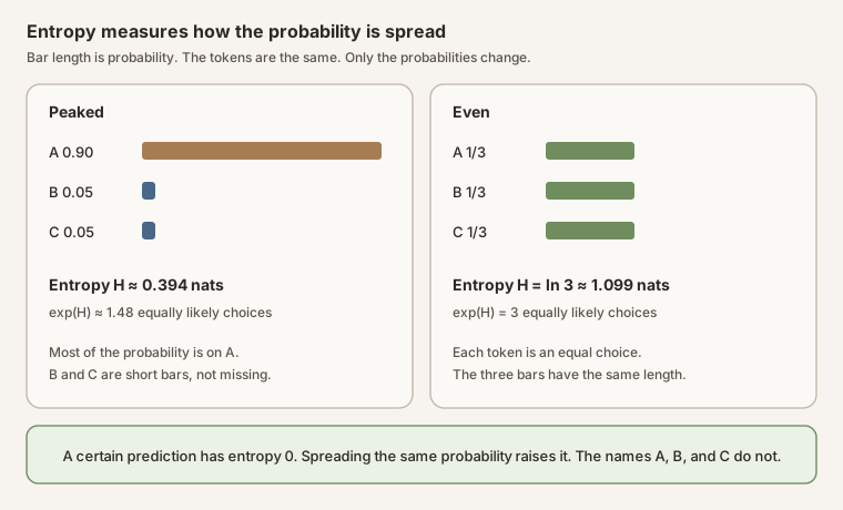
Scroll horizontally to inspect the diagram. The caption below provides a full text explanation.

Worked example

Take probabilities \(0.90\), \(0.05\), and \(0.05\). Each term \(-\,p\ln p\) is about \(0.0948\), \(0.1498\), and \(0.1498\). Their sum is

Then \(e^{0.3944}\approx 1.48\). The prediction is a little more uncertain than a sure choice of one token, and far less uncertain than an even choice of three. That even choice has entropy \(\ln 3\approx 1.099\) nats, and \(e^{\ln 3}=3\).

The same rule in code checks that probabilities are finite and treats a zero probability as a zero contribution:

from math import isfinite, log

def next_token_entropy(probabilities: list[float]) -> float:
    total = sum(probabilities)
    if any(not isfinite(p) or p < 0 for p in probabilities) or not isfinite(total) or abs(total - 1) > 1e-9:
        raise ValueError("probabilities must be finite, nonnegative, and sum to 1")
    return -sum(p * log(p) for p in probabilities if p > 0)

log is the natural logarithm, so the result is in nats. Divide by \(\ln 2\) to report bits, the base-2 unit of information.

One step, not a whole run

The definition applies to one next-token distribution. In an iterative feedback run, which feeds a model-derived representation back as the next input, the model produces a new distribution and therefore a new entropy at every step. Any map or summary must state whether it shows a specified step or an average over steps. On a repeating run, a single-step entropy describes one phase of the cycle; another phase or stopping step can have a different value. For example, the header map of the November note on hiding bits and logic in a language-model feedback loop plots the entropy of a single final measurement step rather than a window average.

What the number does not say

A low entropy says the probability is concentrated. At the mathematical extreme, a distribution that puts probability 1 on one token has entropy zero. Greedy continuation is different: it selects a highest-probability token from whatever distribution it receives, even when that distribution has nonzero entropy (and an implementation must break ties if several tokens share the maximum score). A high entropy says the probability is spread out. Under soft-token feedback, the probabilities are weights in a weighted average of token embeddings, the numeric vectors used to represent tokens. Entropy describes how dispersed those weights are; it does not say how many embeddings have nonzero weight.

Entropy also does not identify which tokens carry the probability. Two distributions can share an entropy and favor different tokens. Nor is it the geometric spread of those tokens’ embedding vectors: the sensitivity of one feedback step depends on how far apart the embedding vectors lie as well as on their probability weights, so a high entropy over similar embeddings is a different fact from a high entropy over very different embeddings.

It is not the perplexity of a text. Perplexity exponentiates the average negative log-probability that the model assigned to the tokens that actually occurred, so it depends on both the predicted distributions and the observed tokens. Next-token entropy ignores the token that came next and scores only the distribution itself. It is also not a Lyapunov exponent. Next-token entropy is measured in nats, whereas a discrete-time Lyapunov exponent computed with natural logarithms is a growth rate in nats per step: it measures how rapidly a tiny perturbation to the state grows or shrinks, not uncertainty over tokens.

See also: nat, temperature, logit, soft-token feedback.