p-value

A p-value answers one precise question:

Under a stated null model, and with the analysis rule fixed in advance, what is the probability of a test statistic at least as incompatible with that null as the one observed?

That conditional probability is not simply “the chance this happened by accident.” Its meaning depends on the null, the statistic, the assumptions, and whether the test is one- or two-sided. In particular, a \(p\)-value measures incompatibility with a specified statistical model; it is not the probability that the null hypothesis is true.

The worked example below is a small language-model (LLM) experiment: you change the prompt text sent to a model and ask whether a chosen vocabulary entry becomes more favored. The same sign-test logic applies to many other paired comparisons; the LLM setting is only the concrete setup used to teach the idea.

Set up the experiment

A large language model is a neural network that, given some input text, assigns a score to every entry in a fixed vocabulary (the model’s list of token strings, which are often subword pieces rather than whole words). Higher score means the model treats that entry as a better next-token candidate at a particular position.

Freeze one model. Then choose:

1. A probe token \(W\): one exact vocabulary entry, including its whitespace and capitalization convention. A displayed English word may map to several tokens, or to different tokens depending on leading space and case, so do not treat “the word” as automatically identical to one vocabulary row. If you truly need several allowed variants, pre-register the exact set and a single scoring rule applied identically in both arms (for example, a fixed canonical token, or the maximum score among that fixed set). Choosing the best-looking variant after seeing the outcomes is selection, not a pre-registered probe. If the target is several tokens long, use a sequence score (worked example just below) rather than ranking only the first piece.
2. Two prompt templates that differ in one intended way:
   • a control prompt: the baseline text, with no intervention;
   • a treatment prompt: the same kind of setup, plus the intervention you want to test (for example, added pressure or threat wording).
3. A battery of fixed test sentences \(S_1,\ldots,S_{16}\). Write them before seeing outcomes and do not edit them afterward.

Multi-token probes in practice. Suppose the surface string is New York and the model’s tokenizer splits it into two vocabulary entries \(w_1\) = New and \(w_2\) = a leading-space York (exact spelling is tokenizer-specific; freeze it). Let \(x\) be the full prompt-plus-sentence prefix where you score. Then:

1. Read the next-token distribution at \(x\) and take \(\log P(w_1\mid x)\), the log-probability of New.
2. Append New to the context, so the prefix is now \(x\) followed by \(w_1\).
3. Read the next-token distribution there and take \(\log P(w_2\mid x,w_1)\), the log-probability of leading-space York.
4. Add those two numbers: \(\log P(w_1\mid x)+\log P(w_2\mid x,w_1)\).

That sum is one scalar per arm. Compare control and treatment with that scalar (or its sign). Ranking New alone would ignore whether York is actually a good continuation after it.

For each test sentence \(S_i\), run the model twice:

• Control arm: control prompt followed by \(S_i\).
• Treatment arm: treatment prompt followed by the same \(S_i\).

For each arm, compute the next-token score distribution immediately after the complete prompt-plus-sentence prefix \(S_i\). Fix in advance the final character, whitespace convention, tokenizer, and that scoring position. That is where you look up the probe token \(W\) chosen above. Other choices are different experiments: scoring \(W\) right after the intervention text, at a blank inside the sentence, as a free continuation after extra generated text, or at a position where \(W\) is already written into the input (so the model is not being asked to prefer \(W\) as the next unseen token).

Only the surrounding prompt changes. The sentence, probe token, model, and scoring rule stay fixed. Those two runs form one matched pair: two measurements on the identical sentence, so later comparisons do not mix different sentences together. Sixteen sentences give sixteen pairs, not thirty-two unrelated runs.

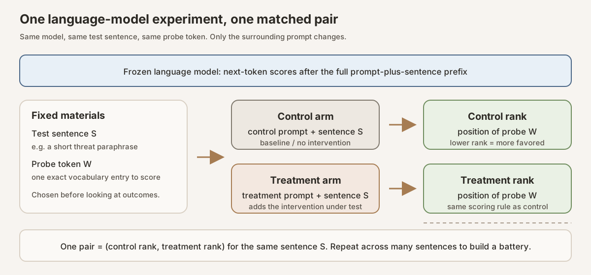
Scroll horizontally to inspect the diagram. The caption below provides a full text explanation.

Turn each pair into a sign

After each run, read the model’s next-token scores over the vocabulary. The probe’s rank is its position in that scored list: rank 1 is the highest-scoring entry, so a lower numerical rank means the probe is more favored under that prompt. Rank is a valid directional summary, but a weak scientific one: a jump from rank 10000 to 100 and a jump from rank 2 to 1 both count as one win, and a tiny log-probability change can move rank a lot when many tokens are tightly packed.

For pair \(i\), this tutorial’s primary signed quantity is the rank gap

Then \(D_i>0\) means the treatment prompt placed the probe at a better (lower) rank than the control prompt did on that same sentence. The sign test discards the size of each nonzero difference and keeps only whether the treatment won or lost that pair. In a real study, prefer also reporting the paired log-probability gap \(\log P_{\mathrm{treatment}}(W\mid S_i)-\log P_{\mathrm{control}}(W\mid S_i)\), choosing one pre-specified primary quantity for the test, and summarizing magnitude with something such as a median difference and interval. Rank can remain a secondary visualization.

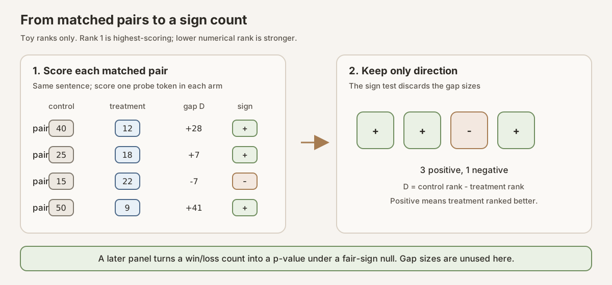
Scroll horizontally to inspect the diagram. The caption below provides a full text explanation.

Where the randomness comes from

If the model is frozen and the sixteen sentences are fixed, each arm’s scores are essentially deterministic computations. The fourteen positive signs are not automatically fourteen independent coin-flip observations created by running the model twice.

The calculation below treats the test sentences as independent units from a specified population of sentences. Under that superpopulation model, and under the null, the nonzero treatment-versus-control differences have independent equiprobable signs. The model outputs themselves are not the source of randomness; the inferential model concerns how the sentence-level signs would vary across that population. If the sixteen sentences are merely a fixed hand-selected battery, the 14/16 count remains a valid descriptive result for that battery, but a binomial \(p\)-value that generalizes beyond it requires additional assumptions (or a design whose randomization supplies the reference distribution). An arbitrarily chosen prompt battery does not earn \(p=0.004\) as a population claim merely by being tallied.

From a win count to a p-value

After dropping ties, suppose the sixteen pairs give 14 positive and 2 negative signs. The null used here is no systematic directional tendency across the target population of sentence-level comparisons: conditional on a difference being nonzero,

and the retained signs are jointly distributed as independent fair signs. Equivalently, every one of the \(2^{16}=65536\) sign patterns is equally likely. That null is not automatically the same as “the prompts are semantically identical,” “the treatment has no effect on every sentence,” “the average rank difference is zero,” or “the model has no preference for the concept associated with \(W\).”

The conventional two-sided exact sign test used here counts a result this lopsided in either direction as extreme: as few as 0–2 wins, or as many as 14–16 wins.

Expanding the low-win tail:

By symmetry, the high-win tail has the same mass: \(P(K\ge 14)=P(K\le 2)\). Doubling one tail (the two-sided step for this symmetric \(p_0=1/2\) binomial) gives

A rounded report of that value is \(p=0.004\). Other discrete two-sided conventions exist; name the one you use.

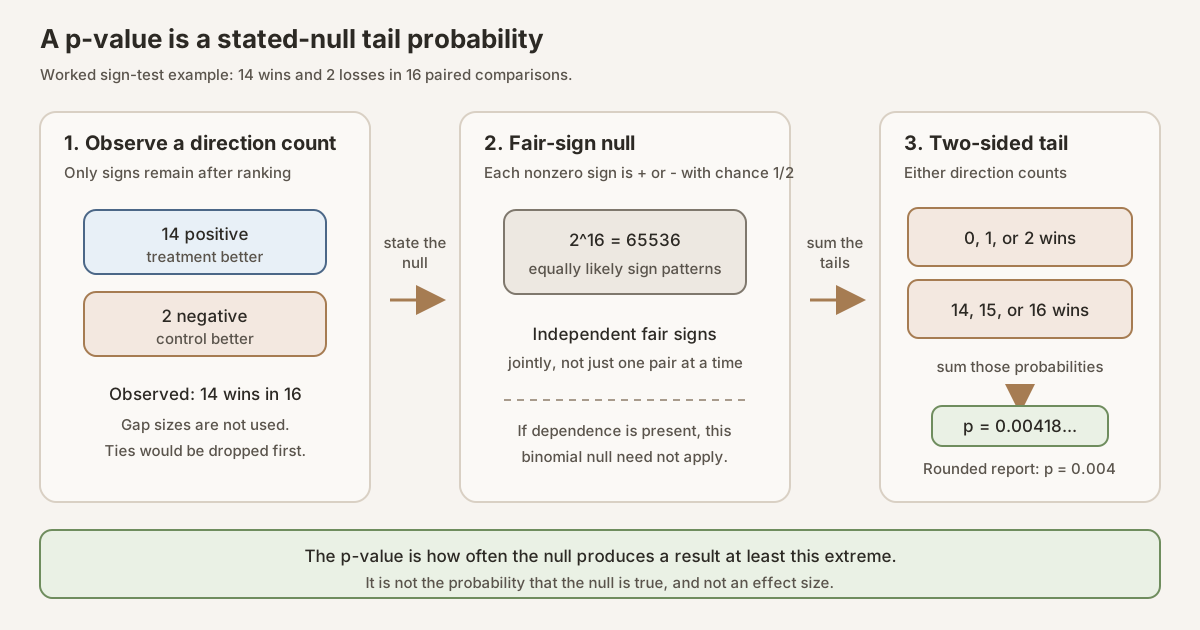
Scroll horizontally to inspect the diagram. The caption below provides a full text explanation.

This dependency-free Python reproduces the calculation:

from math import comb

def sign_test_two_sided(wins: int, losses: int) -> float:
    n = wins + losses
    smaller_tail = sum(
        comb(n, k) for k in range(min(wins, losses) + 1)
    ) / 2**n
    return min(1.0, 2 * smaller_tail)

print(sign_test_two_sided(14, 2))  # 0.004180908203125

With \(n=10\), the same rule gives 10/10 → 0.00195, 9/10 → 0.0215, and 8/10 → 0.109. The discreteness is why a small battery needs an extreme direction count to cross a conventional threshold.

Assumptions and choices

• Pairing: each treatment result must be compared with its genuinely matched control on the same sentence. Unmatched arms do not become valid because their \(p\)-value is small.
• Null distribution: conditional on the number \(n\) of non-ties, the binomial calculation is justified when the retained signs are independent Bernoulli(\(1/2\)), or when the experimental design otherwise induces that same null distribution. Independent fair signs are a standard sufficient condition. Exchangeability of the sentence units alone does not imply independent fair signs. Closely related paraphrases or other dependent units can violate this model; see i.i.d..
• Ties: \(D_i=0\) has no sign. Omit ties and report the reduced effective \(n\), rather than silently counting them as wins or losses.
• Sidedness: choose a one-sided alternative only when its direction was fixed in advance. Otherwise report the conventional two-sided exact result used above.
• Selection: the test does not correct for trying many probes, thresholds, subsets, or analysis rules and reporting the most favorable one.

“Exact” means no large-sample approximation was used to compute the binomial tail. It does not remove these design assumptions. A different exact conditional construction appears in Fisher’s exact test for association in a count table. When the differences have a meaningful ordered magnitude and their distribution can reasonably be treated as symmetric, the Wilcoxon signed-rank test uses the ranks of their absolute magnitudes as well as their signs.

What a p-value does not tell you

A \(p\)-value is not the probability that the hypothesis is true, not an effect size, and not a population estimate. The direction count says how consistently the matched pairs moved. Rank gaps describe movement in vocabulary ordering, but should not be interpreted as interval-scale effect sizes. Neither turns a convenience sample into i.i.d. draws from a wider population.

Prefer the full evidence bundle: the direction count, the exact \(p\), a pre-specified magnitude summary (preferably on a log-probability or other interval-friendly scale), matched treatment/control conditions, and any matched readout baselines used in the study. A tiny \(p\) from a confounded comparison remains a confounded result.

See also: rank, Wilcoxon, Fisher’s exact test, best-rank, i.i.d., prompt echo.

Sources

• ASA Statement on Statistical Significance and P-Values
• NIST: Wilcoxon Signed Rank Test