Knowledge Base / Glossary
Residual stream
The model's running hidden-state channel: each layer reads it, adds an update, and passes it on.
The residual stream is the running hidden state carried through a Transformer, a neural-network architecture that repeatedly combines attention with position-wise transformations. More precisely, there is one residual vector per token position, not one vector for the whole prompt. In the notation below, \(\mathbb{R}\) denotes the set of real numbers and the superscript \(\top\) denotes transpose. At layer \(\ell\), a sequence of \(n\) tokens has a residual-state matrix
\[ H_\ell = \begin{bmatrix} h_{\ell,1}^{\top} \\ \vdots \\ h_{\ell,n}^{\top} \end{bmatrix} \in \mathbb{R}^{n\times d_{\text{model}}}. \]Here \(h_{\ell,t}\in\mathbb{R}^{d_{\text{model}}}\) is a column-vector residual state at token position \(t\) and layer index \(\ell\). Its transpose \(h_{\ell,t}^{\top}\) appears as one row of \(H_\ell\). The model width \(d_{\text{model}}\) is the number of coordinates in each vector.
Each Transformer block reads those vectors and adds updates back into them. A multilayer perceptron (MLP) commonly implements the block’s position-wise feed-forward network (FFN), the sublayer that applies the same learned nonlinear function separately at each token position. In a common pre-normalization block, a normalization module rescales the state according to a specified rule and, depending on the module, may also recenter it. The normalization is applied before each update:
\[ U_\ell = H_\ell + \operatorname{Attention}_\ell(N^{\mathrm{attn}}_\ell(H_\ell)), \qquad H_{\ell+1} = U_\ell + \operatorname{MLP}_\ell(N^{\mathrm{mlp}}_\ell(U_\ell)). \]Here \(U_\ell\) is the intermediate residual matrix after the attention update. The superscript \(\mathrm{attn}\) abbreviates “attention.” The symbols \(N^{\mathrm{attn}}_\ell\) and \(N^{\mathrm{mlp}}_\ell\) denote the typically distinct normalization modules used before the attention and MLP updates, respectively. Attention means the update at one position can depend on other positions allowed by the attention rule. The MLP does not directly mix positions, although it transforms vectors that may already contain attention-gathered context. The linked glossary entry gives its standard and gated forms.
The residual stream is therefore better pictured as a sequence of evolving row vectors than as a single global scratchpad.
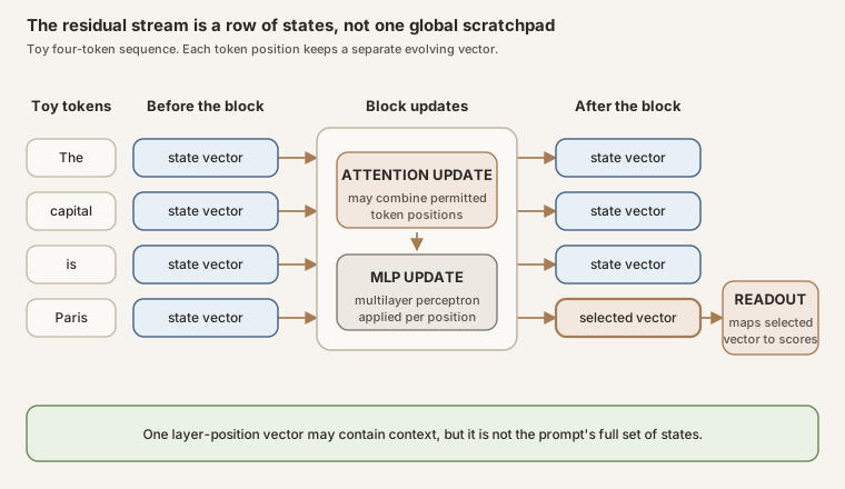
Scroll horizontally to inspect the diagram. The caption below provides a full text explanation.
The, capital, is, and Paris, each of which has a separate vector before the block. Attention can use positions permitted by the architecture’s attention rule, for example current or earlier positions in a causal decoder. The position-wise multilayer perceptron (MLP) then applies the same learned function separately at each position. Four separate vectors continue after the block; the highlighted last-position vector is one selected state from the full residual-state matrix. It may contain contextual information about other positions, but it is not the prompt’s full collection of states. The analyst passes that selected state to a readout, which maps it to derived scores. The diagram omits normalization and explicit residual-addition arrows; the equations in the text show one common pre-normalization arrangement. It is not a universal architecture or tokenizer specification.Worked example
Suppose a tokenizer, the model-specific procedure that maps text to tokens, turns “The capital is Paris” into four tokens. An activation cache is a saved collection of intermediate tensors (multidimensional arrays of values), and cache layouts differ. Assume here that the batch dimension, which indexes input examples, has already been removed. The tensor residual_after has shape (num_blocks, 4, d_model), and residual_after[k] stores \(H_{k+1}\), the state immediately after the block with zero-based index k; consequently, residual_after[k] has shape (4, d_model). Then:
block_index = 20  # the 21st block under zero-based indexing
position = -1     # Python -1 selects the final token position
h = residual_after[block_index, position]  # shape: (d_model,)
If instead a cache stores every boundary from \(H_0\) through \(H_L\) for a model with \(L\) blocks, its first dimension has length \(L+1\), and the state after block_index is residual_boundaries[block_index + 1, position]. Changing position changes the state being inspected. A result at the final prompt position may contain contextual information about earlier permitted positions, but it does not replace the full matrix of position states.
What a readout adds
Mid-network \(h_{\ell,t}\) is a high-dimensional vector, not a sentence in English. Readouts map an analyst-selected state to derived quantities. A logit lens typically applies a specified normalization and the model’s unembedding, the output map to unnormalized vocabulary scores. A Jacobian lens uses a mapping derived from downstream Jacobians, which are matrices of partial derivatives evaluated at specified activations and describe the first-order effect of small activation changes. Its analysis must specify the downstream mapping being differentiated, the source and target activations, and any fitting or averaging protocol.
Scores from these mid-network readouts are derived measurements, not automatically the model’s eventual output. Seeing a word score highly does not by itself show that the model represents a clean, discrete English concept there or that the scored direction causally controls behavior. Causal claims require an intervention and an observed downstream effect.
See also: Transformer, feed-forward network (FFN), multilayer perceptron (MLP), unembedding.