Knowledge Base / Glossary
Root mean square (RMS)
The square root of the mean squared coordinates of a vector, used here as a measure of residual-state scale.
The root mean square (RMS) is a nonnegative scalar that summarizes a real-valued vector’s quadratic coordinate scale. For a nonempty vector \(h\in\mathbb{R}^{d}\),
\[ \operatorname{RMS}(h) = \sqrt{\frac{1}{d}\sum_{i=1}^{d}h_i^2} = \frac{\lVert h\rVert_2}{\sqrt{d}}, \qquad d\ge 1. \]Here \(\mathbb{R}\) is the set of real numbers, \(d\) is the number of coordinates, \(i\) indexes those coordinates, \(h_i\) is coordinate \(i\), and \(\lVert h\rVert_2\) is Euclidean length, the square root of the sum of squared coordinates. RMS is the square root of their quadratic average. Because squaring emphasizes large magnitudes, one unusually large coordinate can strongly affect it.
RMS reports scale, not direction. Negating every coordinate leaves RMS unchanged even though the vector points in the opposite direction.
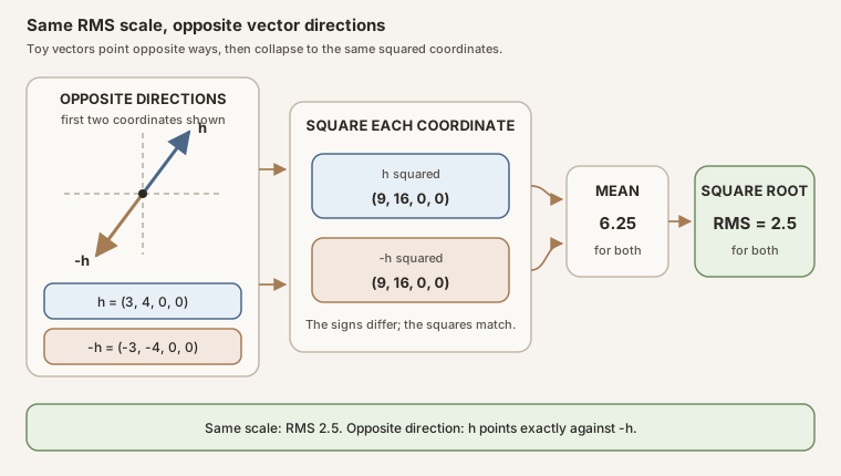
Scroll horizontally to inspect the diagram. The caption below provides a full text explanation.
Worked example and unit-RMS scaling
For \(h=(3,4,0,0)\), the dimension is \(d=4\), so
\[ \operatorname{RMS}(h) = \sqrt{\frac{3^2+4^2+0^2+0^2}{4}} = \sqrt{\frac{25}{4}} =2.5. \]For a nonzero vector, dividing by its RMS produces a unit-RMS vector:
\[ u=\frac{h}{\operatorname{RMS}(h)}, \qquad h\ne 0. \]Then \(\operatorname{RMS}(u)=1\), while its Euclidean length is \(\lVert u\rVert_2=\sqrt{d}\). Unit RMS is therefore different from the usual unit-Euclidean-length convention. An empty vector has no RMS under this definition, and the zero vector cannot be rescaled to unit RMS.
import math

def rms(values):
    if not values:
        raise ValueError("RMS requires at least one coordinate")
    return math.sqrt(sum(x * x for x in values) / len(values))

def unit_rms(values):
    scale = rms(values)
    if scale == 0:
        raise ValueError("the zero vector has no unit-RMS direction")
    return tuple(x / scale for x in values)

h = (3.0, 4.0, 0.0, 0.0)
assert rms(h) == 2.5
u = unit_rms(h)
assert u == (1.2, 1.6, 0.0, 0.0)
assert math.isclose(rms(u), 1.0)
Residual RMS and intervention dose
In these notes, residual RMS means \(\operatorname{RMS}(h)\) for one chosen residual-stream vector, normally at a specified layer and token position. An intervention protocol may state a signed amplitude \(\alpha\) relative to that scale. For a unit-RMS direction \(u\), the requested edit is
\[ e_{\text{requested}} = \alpha\,\operatorname{RMS}(h)\,u, \qquad \operatorname{RMS}(e_{\text{requested}}) = |\alpha|\,\operatorname{RMS}(h). \]If \(\operatorname{RMS}(h)=2\) and the nonnegative dose fraction is \(\alpha=0.03\), the requested edit has RMS \(0.03\times2=0.06\). RMS discards sign, so a signed negative amplitude has the same RMS as its positive counterpart.
Numerical precision can separate a request from what the model receives. A protocol may construct the edit in 32-bit floating point (FP32), a relatively precise computer number format, and then cast, or round, it to bfloat16 (BF16), a coarser 16-bit format used for many model activations. The rounded requested edit and the realized edit, the actual stored state after the intervention minus the corresponding clean state, need not match. Their difference can be material relative to a very small requested dose. A reproducible report should name the numeric formats and state exactly where the realized difference is measured.
RMS versus root-mean-square error
Root-mean-square error (RMSE) applies the RMS calculation to a coordinate-wise difference between a reference vector \(x\) and an approximation \(\hat{x}\):
\[ \operatorname{RMSE}(x,\hat{x}) = \operatorname{RMS}(x-\hat{x}) = \sqrt{\frac{1}{d}\sum_{i=1}^{d}(x_i-\hat{x}_i)^2}. \]Relative RMSE divides that error by a named, nonzero reference size. One convention is
\[ \operatorname{relative\ RMSE}(x,\hat{x}) = \frac{\operatorname{RMSE}(x,\hat{x})}{\operatorname{RMS}(x)}, \qquad \operatorname{RMS}(x)>0. \]Other denominators are possible, including \(\operatorname{RMS}(\hat{x})\). A protocol must state which nonzero reference it uses. RMS alone is a size; RMSE is the size of a mismatch.
RMS is not RMSNorm
Root mean square layer normalization (RMSNorm) is a learned neural-network layer that uses an RMS-like denominator. One common stabilized form is
\[ y_i = g_i \frac{x_i}{\sqrt{\frac{1}{d}\sum_{j=1}^{d}x_j^2+\varepsilon}}, \]where \(x_i\) is input coordinate \(i\), \(g_i\) is a learned per-coordinate gain, \(j\) indexes all \(d\) input coordinates, and \(\varepsilon>0\) protects the denominator from zero. Unlike layer normalization, RMSNorm does not subtract the coordinate mean. The learned gains mean its output need not have unit RMS (Zhang and Sennrich, 2019). A Transformer may use RMSNorm, another normalization rule, or a different placement; none is implied by the scalar RMS definition.
What RMS does not establish
- It is not a probability, confidence, or calibrated uncertainty.
- Equal RMS does not mean equal direction, coordinate pattern, semantics, or causal effect.
- Unit RMS does not make a direction a uniquely interpretable feature.
- RMS is sensitive to large coordinates and does not identify which coordinates produced the scale.
See also: residual stream, Transformer, Jacobian lens.