Knowledge Base / Deep Dives
BF16, FP16, and FP32: Precision, Range, Swamping, and Determinism
A worked Deep Dive on floating-point formats for model arithmetic: bit layouts, GPU Tensor Core support, round-to-nearest demos in PyTorch, accumulation swamping when small adds meet short mantissas, and run-to-run determinism measured across five execution stacks.
On this page 23 sections
Neural-network code stores numbers in floating-point formats: a sign bit, an exponent that largely controls range, and a significand that controls precision. The stored low-order portion is the fraction field, informally also called the mantissa. Shorter formats use less storage per element and can reduce memory traffic. They can also run faster when the hardware and software provide an accelerated path, but emulated or conversion-heavy paths may be slower.
This Deep Dive compares three common data types (dtypes):
- FP32: 32-bit floating point (also called float32 or F32)
- FP16: 16-bit floating point (also called float16 or F16; IEEE 754 binary16)
- BF16: bfloat16 (brain floating point)
A short glossary entry lives at BF16, FP16, and FP32. This page carries the worked demos, the swamping chart, and the hardware / determinism detail.
Choose a reading route.
- Learning the formats: begin with bit layouts, range and spacing, and the worked demo.
- Choosing a format: read when to use each format and hardware support, keeping the limits of a format label in view.
- Investigating repeatability: jump to matrix-multiplication repeatability, then the measured case study and receipts and scripts.
How the bits are spent
Mixed precision means using more than one numeric format in a computation, such as FP16 operands with FP32 accumulation. A master weight is a higher-precision copy of a trainable parameter retained for optimizer updates.
| Name | Also called | Bits | Exponent bits | Trailing significand bits | Typical role |
|---|---|---|---|---|---|
| FP32 | float32, F32, single | 32 | 8 | 23 | Reference / CUDA-core math, loss, some master weights |
| FP16 | float16, F16, half | 16 | 5 | 10 | Mixed precision; narrower range than FP32 |
| BF16 | bfloat16, brain float | 16 | 8 | 7 | Activations / matrix multiplications (matmuls); FP32-like range, less precision |
| TF32 | TensorFloat-32 | FP32 storage; 19 effective input bits for multiplication (1 sign, 8 exponent, 10 trailing fraction) | 8 | 10 | NVIDIA Tensor Core compute mode; FP32 inputs are rounded for multiplication, commonly with FP32 accumulation |
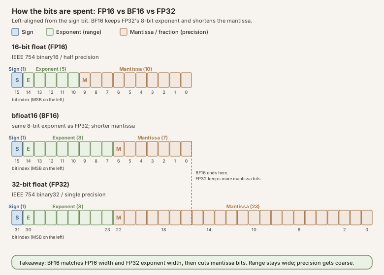
Scroll horizontally to inspect the diagram. The caption below provides a full text explanation.
Rough intuition:
- FP32 is the familiar high-precision baseline. For a normal finite binary value, the encoding supplies an implicit leading 1, so FP32 has 24 bits of precision.
- FP16 spends more of its 16 bits on precision and fewer on range (max finite FP16 is 65504). Normal FP16 values have 11 bits of precision.
- BF16 keeps FP32’s 8-bit exponent and only 7 trailing fraction bits, so normal BF16 values have 8 bits of precision.
- TF32 is an NVIDIA Tensor Core compute mode rather than a storage dtype: FP32 operands are rounded to 10 trailing fraction bits for multiplication while retaining FP32-like range.
One standards note: FP32 and FP16 are IEEE 754 interchange formats (binary32 and binary16). BF16 and TF32 are not; they are industry/vendor formats that borrow IEEE-style encoding conventions. Defer to each vendor’s documentation for their exact edge-case behavior.
Numerical range and spacing
The range is symmetric for negative finite values. “Smallest positive normal” is where normal encoding begins; subnormal values extend closer to zero with reduced effective precision. “Spacing above 1” is the gap from 1 to the next larger representable value.
| Storage format | Largest finite value | Smallest positive normal | Smallest positive subnormal | Spacing above 1 |
|---|---|---|---|---|
| FP32 | \(3.4028235\times10^{38}\) | \(1.1754944\times10^{-38}\) | \(1.4012985\times10^{-45}\) | \(1.1920929\times10^{-7}\) |
| FP16 | \(65504\) | \(6.1035156\times10^{-5}\) | \(5.9604645\times10^{-8}\) | \(9.765625\times10^{-4}\) |
| BF16 | \(3.3895314\times10^{38}\) | \(1.1754944\times10^{-38}\) | \(9.1835496\times10^{-41}\) | \(7.8125\times10^{-3}\) |
Normal versus subnormal
A normal floating-point number uses a nonzero exponent field. For a finite binary normal, the leading significand bit is understood to be 1 even though that bit is not stored:
\[ \text{normal significand}=1.\text{fraction bits}. \]That implicit leading 1 gives one extra bit of precision without consuming a
stored bit. BF16 stores only the 7 bits after the binary point. For a normal
value, the decoder supplies the leading 1 automatically:
stored fraction bits:       abcdefg
decoded significand:      1.abcdefg
The decoded significand therefore contains 8 meaningful binary digits: 1 known leading bit plus 7 stored fraction bits. This is why BF16 has 8 bits of significand precision, even though its bit layout contains only 7 fraction bits. It does not secretly store an eighth fraction bit.
A subnormal number is a nonzero value with an all-zero exponent field. It does not receive the implicit leading 1:
\[ \text{subnormal significand}=0.\text{fraction bits}. \]The same 7 BF16 fraction bits are stored, but the decoder supplies a leading
0 instead of a leading 1:
stored fraction bits:       abcdefg
decoded significand:      0.abcdefg
That leading 0 is not a meaningful precision bit. The first 1 must come
from somewhere inside the stored fraction. As a subnormal gets smaller, that
first 1 moves farther right:
larger subnormal:          0.1010000
smaller subnormal:         0.0000001
The larger example has several meaningful binary digits after its first 1.
The smallest positive BF16 subnormal has only the final stored 1, so it has
just one meaningful significand bit. In other words, subnormals retain the
format’s fixed spacing near zero, but their relative precision decreases
as they approach zero.
Subnormals fill the gap between the smallest positive normal value and zero. Instead of jumping directly from the smallest normal number to zero, the format represents progressively smaller values with progressively fewer meaningful precision bits. This behavior is called gradual underflow.
For a concrete FP16 example:
- smallest positive normal: \(2^{-14}\approx 6.10\times10^{-5}\);
- smallest positive subnormal: \(2^{-24}\approx 5.96\times10^{-8}\);
- anything smaller than the rounding boundary near that minimum becomes zero.
The table describes what each format can represent. A particular accelerator or kernel may use flush to zero, treating subnormal inputs or results as zero for performance. Therefore, format-level subnormal support does not by itself prove that every hardware path preserves those values.
This table exposes the main tradeoff: BF16 reaches almost as far as FP32, but its spacing near 1 is 8192 times coarser. FP16 has finer spacing than BF16 near 1, but its largest finite value is only 65504.
Are FP8 and FP4 real?
Yes, but neither name identifies one universal format:
- FP8 commonly means an E4M3 variant (more precision, less range) or an E5M2 variant (less precision, more range). Exact treatment of infinities, not-a-number values, and unsigned-zero variants depends on the named format.
- FP4 commonly uses a very small encoding such as E2M1. In practical model kernels it is often paired with per-block scale factors, so the encoding’s raw four-bit range is not the tensor’s effective numerical range.
They matter for specialized training and inference on recent accelerators, but including them in the main three-format table would imply false interchangeability. A reproducible protocol should name the exact variant, scaling granularity, scale dtype, accumulation dtype, hardware path, and framework implementation. This Deep Dive keeps FP8/FP4 as context and focuses its worked examples on FP32, FP16, and BF16.
When to use each format
This is a starting guide, not a substitute for checking the exact model, operation, hardware, and framework path. In mixed-precision systems, storage, multiplication, and accumulation may use different formats.
| Format | Good fit when | Avoid or reconsider when | Main tradeoff |
|---|---|---|---|
| FP32 | Establishing a reference result; debugging numerical behavior; computing precision-sensitive reductions, metrics, losses, or optimizer state; the workload is small enough that memory and throughput are secondary | A validated lower-precision path gives acceptable results and the workload is limited by accelerator throughput or memory capacity | Highest precision of these three, but twice the storage and memory traffic of FP16/BF16 and often lower Tensor Core throughput |
| FP16 | The accelerator has a strong native FP16 path (including older Turing hardware such as T4); values stay within FP16’s narrower range; its extra significand precision over BF16 matters; training uses an appropriate mixed-precision and loss-scaling recipe | Values may exceed 65504 or become extremely small; overflow/underflow is already visible; the workload naturally prefers BF16; assuming loss scaling fixes every numerical issue | More precision near a fixed magnitude than BF16, but much less exponent range than BF16/FP32 |
| BF16 | Training or inference on Ampere-or-newer hardware with native BF16 support; FP32-like dynamic range is valuable; model activations or weights tolerate coarser spacing; avoiding FP16 overflow is more important than preserving FP16’s extra fraction bits | Small updates or differences must survive beside larger values; precision-sensitive accumulation is stored in BF16; the device lacks a native BF16 fast path (for example T4); a measured quality or fidelity check fails | FP32-like range in 16 bits, but only 7 stored fraction bits, so rounding and swamping happen sooner |
A practical default on modern training accelerators is often BF16 operands or activations with FP32 accumulation, not “everything in BF16.” On T4, FP16 is usually the native 16-bit Tensor Core choice. Keep an FP32 reference path and validate the actual task metric before treating either 16-bit format as safe.
GPU Tensor Cores
A card can usually store or emulate many dtypes. What changes in practice is whether Tensor Cores (specialized matrix units) natively accelerate that format, or whether execution uses general-purpose GPU arithmetic lanes (CUDA cores) or casting / software emulation.
| GPU generation (examples) | Fast Tensor Core highlights | Practical note |
|---|---|---|
| Turing (Tesla T4, RTX 20-series) | FP16, INT8, INT4; FP32 on CUDA cores | No native BF16 Tensor Cores. |
| Ampere (A100, RTX 30-series) | Adds BF16 (and TF32) | Common sweet spot for BF16 large-model runs. |
| Ada (L40, RTX 40-series) | FP8, FP16, BF16, TF32 | Check the exact stock-keeping unit (SKU). |
| Hopper (H100, …) | FP8, FP16, BF16, TF32 | Throughput and software paths differ from Ada. |
T4 is not “unable to do full precision.” It has FP32 CUDA-core throughput; it lacks native BF16 Tensor Core acceleration.
Worked demo in PyTorch
The demos below use PyTorch, a tensor and neural-network
framework. A tensor is a multidimensional array of numbers (here often a
length-1 vector). torch.tensor([v], dtype=...) builds such an array from
Python values and stores it in the named floating-point format; .item() reads
the single scalar back out as an ordinary Python number for printing. Calling
.to(torch.float16) or .to(torch.bfloat16) casts (converts) the tensor
into that format, with the target format’s rounding rules.
The demos intentionally store every partial sum in the selected format. That is not a model of every matrix-multiplication kernel: FP16 and BF16 Tensor Core general matrix multiplication (GEMM) operations commonly multiply low-precision operands while accumulating products in FP32.
These conversions use round to nearest, ties to even: choose the nearest representable value, and when the input is exactly halfway between two values, choose the one whose least-significant retained significand bit is 0.
Reproduce the numeric receipt and refresh the chart by downloading
reproduce.py (published beside this page) and running:
uv run reproduce.py
1. Hardware check
Ask the runtime which GPU is present and what PyTorch reports about it. Be
precise about what the probe proves: torch.cuda.is_bf16_supported() reports
BF16 dtype support (it even accepts an including_emulation argument),
not proof that BF16 work will dispatch to native Tensor Cores. Whether a
given kernel actually uses the matrix units depends on the architecture, the
library, and the dispatch path, so print the device identity separately and
check it against the vendor’s architecture tables:
import torch

if torch.cuda.is_available():
    print(f"GPU: {torch.cuda.get_device_name(0)}")
    print(f"Compute capability: {torch.cuda.get_device_capability(0)}")
    print(f"BF16 dtype support reported: {torch.cuda.is_bf16_supported()}")
else:
    print("Running on CPU.")
Example output (A100 Colab):
GPU: NVIDIA A100-SXM4-40GB
Compute capability: (8, 0)
BF16 dtype support reported: True
The A100’s compute capability 8.0 (Ampere) is what places it in the native
BF16 Tensor Core generation; the dtype probe alone would also return True
on devices that support BF16 through emulation. The later dtype demos do
not require any GPU; they are cast arithmetic.
2. Precision near 1.0
Cast three nearby values through FP32, FP16, and BF16. BF16 collapses all three to 1.0. FP16 keeps \(1 + 2^{-10}\) but rounds \(1 + 2^{-12}\) to 1.0.
print("--- Precision Check: Adding small values to 1.0 ---")
vals = [1.0, 1.0 + 2**-12, 1.0 + 2**-10]
for v in vals:
    t_fp32 = torch.tensor([v], dtype=torch.float32)
    t_fp16 = t_fp32.to(torch.float16)
    t_bf16 = t_fp32.to(torch.bfloat16)
    print(
        f"Input: {v:<15} | FP32: {t_fp32.item():<15} | "
        f"FP16: {t_fp16.item():<15} | BF16: {t_bf16.item():<15}"
    )
--- Precision Check: Adding small values to 1.0 ---
Input: 1.0             | FP32: 1.0             | FP16: 1.0             | BF16: 1.0
Input: 1.000244140625  | FP32: 1.000244140625  | FP16: 1.0             | BF16: 1.0
Input: 1.0009765625    | FP32: 1.0009765625    | FP16: 1.0009765625    | BF16: 1.0
None of those inputs is an exact tie, so they exercise only the “nearest” half of round-to-nearest, ties-to-even. To see the tie rule itself, feed each format a value exactly halfway between 1.0 and its next representable neighbor: \(1 + 2^{-11}\) for FP16 (halfway to \(1 + 2^{-10}\)) and \(1 + 2^{-8}\) for BF16 (halfway to \(1 + 2^{-7}\)). Both round down to 1.0 because, of the two equally distant candidates, 1.0 is the one whose last retained significand bit is 0 (even):
print("--- Ties-to-even Check ---")
fp16_tie = torch.tensor([1.0 + 2**-11], dtype=torch.float32)
bf16_tie = torch.tensor([1.0 + 2**-8], dtype=torch.float32)
print(f"FP16 tie 1 + 2^-11: {fp16_tie.to(torch.float16).item()}")
print(f"BF16 tie 1 + 2^-8:  {bf16_tie.to(torch.bfloat16).item()}")
--- Ties-to-even Check ---
FP16 tie 1 + 2^-11: 1.0
BF16 tie 1 + 2^-8:  1.0
3. Swamping under cast-at-each-step accumulation
Now add \(10^{-4}\) ten thousand times, casting the increment and the running sum after every step:
\[ s \leftarrow \mathrm{cast}\bigl(s + \mathrm{cast}(10^{-4})\bigr). \]When a small addend cannot change a larger rounded sum, that loss is called swamping (also absorption): the short mantissa cannot resolve the increment once the sum’s unit in the last place sits above the edit. The term is standard in numerical computing and in the reduced-precision deep-learning literature; Wang et al. (2018) use it for exactly this full-absorption failure in low-precision training accumulations, and Osorio et al. (2022) measure how often it occurs in BF16 fused multiply-add units (see References).
To be precise about what is being demonstrated: this is low-precision storage with cast-at-each-step accumulation, not “BF16 accumulation” in general. Vendor-accelerated GEMM paths typically take BF16 or FP16 inputs and accumulate in FP32, which avoids exactly this failure.
print("--- Accumulation Swamping Demo ---")
n_steps = 10000
step_val = 1e-4

fp32_sum = torch.tensor([0.0], dtype=torch.float32)
fp16_sum = torch.tensor([0.0], dtype=torch.float16)
bf16_sum = torch.tensor([0.0], dtype=torch.bfloat16)
fp32_history, fp16_history, bf16_history = [], [], []

for _ in range(n_steps):
    fp32_sum = (fp32_sum + torch.tensor([step_val], dtype=torch.float32)).to(
        torch.float32
    )
    fp16_sum = (fp16_sum + torch.tensor([step_val], dtype=torch.float16)).to(
        torch.float16
    )
    bf16_sum = (bf16_sum + torch.tensor([step_val], dtype=torch.bfloat16)).to(
        torch.bfloat16
    )
    fp32_history.append(fp32_sum.item())
    fp16_history.append(fp16_sum.item())
    bf16_history.append(bf16_sum.item())

print(
    "Final Sums (Target 1.0): "
    f"FP32={fp32_sum.item():.5f}, "
    f"FP16={fp16_sum.item():.5f}, "
    f"BF16={bf16_sum.item():.5f}"
)
--- Accumulation Swamping Demo ---
Final Sums (Target 1.0): FP32=1.00005, FP16=0.25000, BF16=0.03125
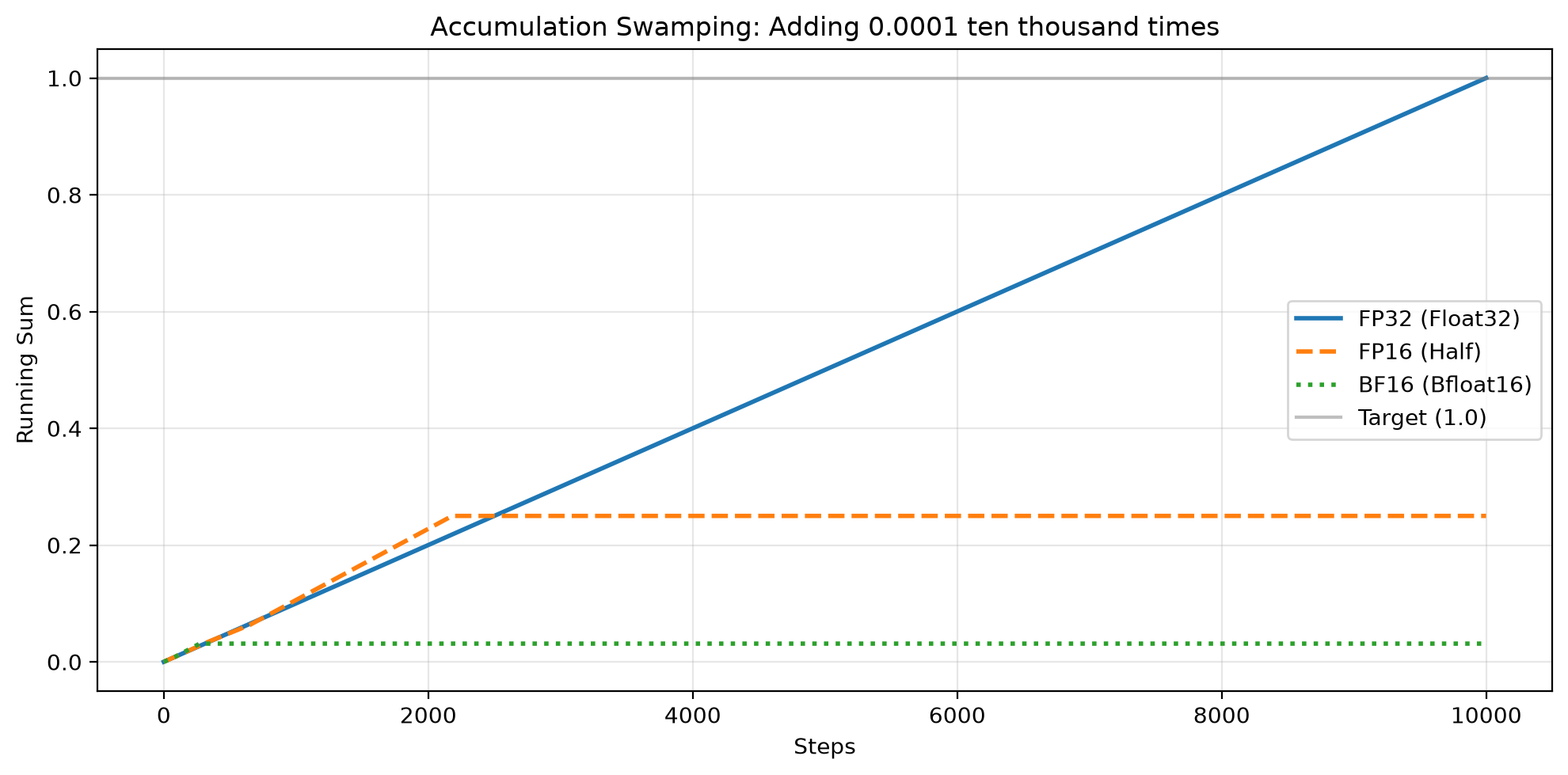
Scroll horizontally to inspect the diagram. The caption below provides a full text explanation.
The figure above is produced by the same plotting code (saved instead of
plt.show()):
import matplotlib.pyplot as plt

plt.figure(figsize=(10, 5))
plt.plot(fp32_history, label="FP32 (Float32)", linewidth=2)
plt.plot(fp16_history, label="FP16 (Half)", linewidth=2, linestyle="--")
plt.plot(bf16_history, label="BF16 (Bfloat16)", linewidth=2, linestyle=":")
plt.axhline(1.0, color="gray", linestyle="-", alpha=0.5, label="Target (1.0)")
plt.title("Accumulation Swamping: Adding 0.0001 ten thousand times")
plt.xlabel("Steps")
plt.ylabel("Running Sum")
plt.legend()
plt.grid(True, alpha=0.3)
plt.tight_layout()
plt.savefig("fig-accumulation-swamping.png", dpi=200, bbox_inches="tight")
4. Overflow / range
FP16’s narrower exponent overflows at \(10^5\). BF16 stays finite (here 99840.0 after rounding).
print("--- Overflow Limit Check ---")
large_val = 1e5
print(
    "FP16 converting 100,000: "
    f"{torch.tensor([large_val], dtype=torch.float16).item()}"
)
print(
    "BF16 converting 100,000: "
    f"{torch.tensor([large_val], dtype=torch.bfloat16).item()}"
)
--- Overflow Limit Check ---
FP16 converting 100,000: inf
BF16 converting 100,000: 99840.0
The 99840 is worth deriving once by hand. Near \(10^5\) the exponent is \(e = 16\) (since \(2^{16} = 65536 \le 10^5 < 2^{17}\)), so adjacent BF16 values are spaced \(2^{16-7} = 512\) apart. The representable neighbors of 100000 are \(195 \times 512 = 99840\) and \(196 \times 512 = 100352\), at distances 160 and 352. Nearest wins: 99840.
Why this matters for interventions
Casting an edit coordinate to BF16 rounds it to a nearby representable value. Separately, when a small edit is added to a larger BF16 activation, swamping can produce zero realized change even though the cast edit was nonzero. Protocols that compare a requested FP32 edit with a realized post-write difference are checking that full write path.
When these notes say BF16 activations, they mean intermediate tensors (multidimensional arrays) intercepted by an instrumentation hook had BF16 storage dtype at the observation or write point. The label does not by itself identify the multiplication, reduction, or accumulation precision used to produce those tensors.
cuBLAS and bit-wise determinism
Scope note: everything in this section, and the measurements on this page, concern the NVIDIA/PyTorch stack our Research Notes run on. These are library-scoped and condition-scoped statements, not universal GPU laws. Other vendors publish analogous but different reproducibility conditions: AMD’s rocBLAS ties bitwise reproducibility to an identical GFX target instruction set, a single HIP stream per handle, an identical ROCm version, and disallowed atomics, while Intel’s oneMKL offers conditional numerical reproducibility for selected BLAS level-3 routines on GPUs with the same product name (see References). We have not tested those stacks; check the vendor tables before transferring any claim here.
cuBLAS is NVIDIA’s Compute Unified Device Architecture (CUDA)-platform implementation of Basic Linear Algebra Subprograms (BLAS) and sits behind many matmul / GEMM calls in PyTorch. For a fixed CUDA toolkit version, cuBLAS documents bitwise reproducibility for supported routines on GPUs with the same architecture and the same number of streaming multiprocessors (SMs), with documented exceptions (concurrent streams, atomics). That is an operation-level guarantee, not whole-experiment reproducibility.
The workspace variable is only needed on older stacks. For years,
deterministic mode raised a RuntimeError from torch.mm, torch.mv, and
torch.bmm on CUDA 10.2+ unless CUBLAS_WORKSPACE_CONFIG=:4096:8 (or
:16:8) was set before CUDA initialized. Modern PyTorch allocates cuBLAS
workspaces explicitly, one per handle/stream combination
(pytorch/pytorch #85447),
which satisfies cuBLAS’s documented reproducibility conditions by itself, so
the requirement check was removed
(pytorch/pytorch #161749).
On a current stack, cuBLAS GEMMs through PyTorch are deterministic without
the variable.
If you run an older PyTorch, still set the variable before CUDA initializes:
import os
os.environ["CUBLAS_WORKSPACE_CONFIG"] = ":4096:8"  # before CUDA init
import torch
torch.use_deterministic_algorithms(True)
torch.backends.cudnn.deterministic = True
torch.backends.cudnn.benchmark = False
torch.backends.cuda.matmul.allow_tf32 = False   # legacy TF32 control
Even in “FP32” matmuls, Ampere+ GPUs may use TF32 Tensor Cores unless
disabled. On current PyTorch, prefer the newer precision controls over the
legacy allow_tf32 flag, and do not mix the two families:
# Current API: request true IEEE FP32 matmuls (disables TF32 downgrades).
torch.set_float32_matmul_precision("highest")
Disabling TF32 is a precision choice with a real throughput cost on Ampere-class matrix units; record which setting produced any number you publish.
Verifying cuBLAS determinism on your stack
Because these requirements move between versions, the reliable move is to
probe the stack you actually run on. We verified the statements above on
PyTorch 2.11.0+cu128 with one A100. Full script:
cublas_determinism_protocol.py;
receipt.
Why the test needs subprocesses. cuBLAS reads CUBLAS_WORKSPACE_CONFIG
when CUDA initializes, which in a notebook happens the first time any tensor
touches the GPU. After that, changing the variable does nothing. So a single
process cannot honestly compare “variable set” against “variable absent.”
The script launches one fresh copy of itself per condition, each with a
controlled environment, and every worker records the variable it actually
saw, so the receipt proves which condition ran:
def launch(condition, workspace):
    env = os.environ.copy()
    env.pop("CUBLAS_WORKSPACE_CONFIG", None)   # start clean
    if workspace:
        env["CUBLAS_WORKSPACE_CONFIG"] = workspace
    env["COND"] = condition
    proc = subprocess.run(
        [sys.executable, os.path.abspath(__file__)],
        env=env, capture_output=True, text=True, timeout=600,
    )
    return json.loads(proc.stdout.strip().splitlines()[-1])
The inputs and the comparison. As in the grid_sample case study below,
the two 2048x2048 FP32 matrices are generated once on the CPU from a fixed
seed, so every condition multiplies identical bytes. Each measuring
condition runs 20 trials and compares all 190 trial pairs bit-for-bit
(outputs viewed as int32), never a scalar summary:
def all_pairs_stats(results):
    max_div, exact, total = 0.0, 0, 0
    for r1, r2 in itertools.combinations(results, 2):
        total += 1
        if torch.equal(r1.view(torch.int32), r2.view(torch.int32)):
            exact += 1
        max_div = max(max_div, (r1 - r2).abs().max().item())
    return {"pairs": total, "exact_pairs": exact, "max_div": max_div}
Condition 1: the probe. Turn on deterministic mode, run one torch.mm,
and record whether PyTorch raises. On an old stack this raises with a
message naming CUBLAS_WORKSPACE_CONFIG; on a current stack it completes:
torch.use_deterministic_algorithms(True)
try:
    _ = a @ b            # torch.mm through cuBLAS
    out["probe"] = "completed"
except RuntimeError as error:
    out["probe"] = "raised"
Condition 2: deterministic-mode repeatability. With the variable set and deterministic mode on, run 20 multiplies and check that every pair is bit-identical. This is the positive control.
Condition 3: the stress arm. Allow nondeterministic algorithms, leave the variable unset, and issue GEMMs concurrently from four CUDA streams, because NVIDIA’s reproducibility note scopes cuBLAS’s guarantee to same-stream use. If shared-workspace effects were going to appear anywhere, it would be here:
torch.use_deterministic_algorithms(False)
streams = [torch.cuda.Stream() for _ in range(4)]
for _ in range(20):
    outputs = [None] * 4
    for i, stream in enumerate(streams):
        with torch.cuda.stream(stream):
            outputs[i] = a @ b
    for stream in streams:
        stream.synchronize()
    results.append(outputs[0].clone())
The results (PyTorch 2.11.0+cu128, one A100-SXM4-80GB, FP32):
| Condition | Deterministic mode | CUBLAS_WORKSPACE_CONFIG |
Outcome |
|---|---|---|---|
| Probe | on | absent | completed, no RuntimeError |
| Probe | on | :4096:8 |
completed |
| Repeatability | on | :4096:8 |
190/190 pairs bit-identical, max divergence 0 |
| Stress (4 streams) | off | absent | 190/190 pairs bit-identical, max divergence 0 |
| Stress (4 streams) | off | :4096:8 |
190/190 pairs bit-identical, max divergence 0 |
Exactly as the PyTorch pull requests document: the probe completes without the variable, and every measured condition is bit-identical, including the concurrent four-stream arm with the variable unset.
Note the contrast with the grid_sample case study below, which uses the
same stack and the same flags. Turning deterministic mode off means “no
guarantee,” not “guaranteed drift.” The flag only controls which
implementations PyTorch may select; what decides the outcome is how the
selected kernel accumulates. A cuBLAS GEMM reduces each output tile in a
fixed order baked into the kernel, so repeated runs retrace the same
additions and produce the same bits even when nondeterministic algorithms
are permitted. The grid_sample backward kernel scatters contributions into
shared coordinates with atomic additions, so its addition order varies run
to run and its rounded sums differ. The determinism registry is
per-operation, and its requirements move between versions, so probe the
stack you actually run on and record the PyTorch, CUDA, and cuBLAS versions
in the receipt. The stress arm’s stability is an observation under this
load pattern, not a proof that shared-workspace nondeterminism is
impossible.
Three general determinism lessons
cuBLAS covers BLAS operations such as matrix multiplication; libcublas is
the shared-library binary that provides that implementation. Many other CUDA
tensor operations use framework or library-specific kernels instead. A cuBLAS
reproducibility setting therefore does not govern every operation in a model.
Across GPU libraries and frameworks, three broader lessons apply:
- Two identical outputs do not prove determinism. A CUDA reduction may use
atomic additions, where many threads update shared destinations and the
effective addition order is not guaranteed. Two lightly loaded runs can
happen to use the same order and produce the same bits. That observed
agreement is evidence about those two runs, not a reproducibility
guarantee under another load, launch configuration, software version, or
device. Also compare the full output or gradient tensor, not only a
scalar summary such as
gradient.sum().item(). Positive and negative coordinate-level differences can cancel in a sum, making two unstable tensors appear identical. A stronger check compares the underlying tensor bits and reports the maximum elementwise difference and number of changed coordinates. - Deterministic mode can change the algorithm and the answer.
torch.use_deterministic_algorithms(True)asks PyTorch to use a documented deterministic implementation when one is available. That implementation may perform reductions or other operations in a different order. Because floating-point addition is not associative, a deterministic result can differ slightly while still processing the same inputs. Do not claim a specific replacement algorithm unless pinned source code or a profiler trace establishes that implementation detail. - Unsupported operations fail closed by default. If PyTorch knows that an
operation has no deterministic implementation for the active device and
mode, deterministic mode raises
RuntimeErrorrather than silently running the known nondeterministic path. Passingwarn_only=Truerequests warnings instead. This check is valuable, but it is not a proof that an entire program is reproducible.
See PyTorch’s version-specific
torch.use_deterministic_algorithms
documentation for the current operation list. Always record the PyTorch,
CUDA, cuDNN, and cuBLAS versions because implementation choices and supported
deterministic paths can change.
Case study: one kernel, five stacks
To make the lessons concrete, we measured run-to-run divergence of one
operation that PyTorch itself classifies as nondeterministic on CUDA:
the backward pass of torch.nn.functional.grid_sample (2D bilinear), whose
input-gradient kernel accumulates many contributions into the same input
coordinates with atomic additions.
The protocol (full script:
divergence_protocol.py):
- All input tensors were generated once on CPU from a fixed seed and transferred, so every device and arm consumed identical bytes.
- The input stayed fixed at 32x32 while the output grid grew from 16x16 to 512x512, increasing how many output samples land on each input coordinate.
- Each geometry was warmed up once, then run 30 times; all 435 trial pairs were compared bit-for-bit (gradients viewed as int32), recording the exact-match rate, the maximum number of drifting coordinates, and the maximum elementwise difference. No scalar summaries.
- Two arms: idle, and a background-matmul condition (four CUDA streams of 4096x4096 FP32 matmuls with stream-local synchronization).
- A final probe enables deterministic mode and records how PyTorch classifies the operation on that stack.
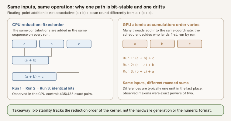
Scroll horizontally to inspect the diagram. The caption below provides a full text explanation.
Results on PyTorch 2.11.0 / CUDA 12.8 (Google Colab, FP32, receipt):
| Device | Compute capability | 512x512 output: drifting coordinates (of 3072) | Max pairwise divergence | Deterministic-mode probe |
|---|---|---|---|---|
| CPU control | n/a | 0 (100% exact pairs at every size) | 0 | completes |
| Tesla T4 (Turing) | 7.5 | 2888 | \(4.20\times10^{-5}\) | raises RuntimeError |
| A100 (Ampere) | 8.0 | 2945 | \(6.10\times10^{-5}\) | raises RuntimeError |
| L4 (Ada) | 8.9 | 2917 | \(4.39\times10^{-5}\) | raises RuntimeError |
| RTX PRO 6000 (Blackwell) | 12.0 | 2933 | \(4.96\times10^{-5}\) | raises RuntimeError |
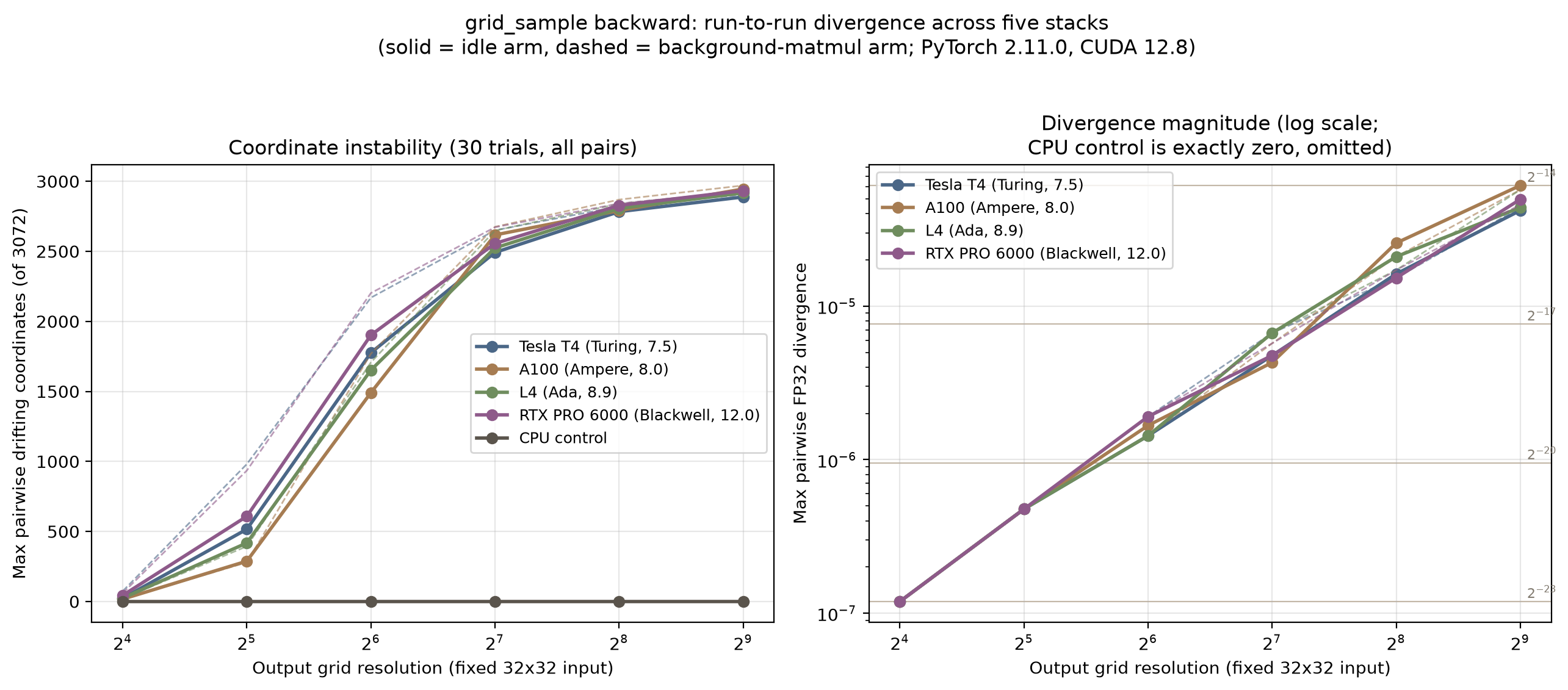
Scroll horizontally to inspect the diagram. The caption below provides a full text explanation.
What this case study establishes, and what it does not:
- The nondeterminism belongs to the kernel, not the hardware. Four GPU generations drift almost identically; the CPU implementation of the same operation on the same bytes is exactly stable. The variable is the execution model (atomic accumulation versus a fixed reduction order).
- The empirical arms and the framework’s registry agree. Every CUDA
device rejected the backward pass under deterministic mode with
grid_sampler_2d_backward_cuda does not have a deterministic implementation; the CPU path completed. - Divergences are ULP-scale. Reordered additions change results by about
one unit in the last place per coordinate, which is also why a scalar
summary such as
grad.sum()can hide thousands of drifting coordinates through cancellation (lesson 1 above). - It does not establish that background load increases drift, that other operations behave the same way, or that these curves hold on other PyTorch/CUDA versions. It also does not identify the kernel’s exact scheduling behavior; that would require pinned source or a profiler trace.
What a format label does not establish
- It does not name the full mixed-precision recipe.
- It does not imply FP16 and BF16 are interchangeable, or that T4 “cannot do FP32.”
- The cast-every-step swamping loop is not a universal law of BF16 kernels.
- Bit layouts follow usual Institute of Electrical and Electronics Engineers (IEEE)-style / industry conventions; defer to framework dtype docs for subnormals, not-a-number (NaN), and rounding mode.
See also: BF16 glossary entry, matmul, root mean square (RMS), residual stream.
References
Standards and formats
- IEEE (2019). IEEE 754-2019: IEEE Standard for Floating-Point Arithmetic. The normative source for binary32 / binary16 encodings, subnormals, rounding modes, and ties-to-even. BF16 and TF32 are not IEEE 754 interchange formats.
- Open Compute Project (2023). OCP Microscaling (MX) Formats Specification. Block-scaled low-bit formats (including FP4/E2M1 variants) referenced in the FP8/FP4 discussion.
Vendor documentation
- NVIDIA. Floating Point and IEEE 754 Compliance for NVIDIA GPUs. CUDA rounding behavior, FMA, flush-to-zero controls, and IEEE-compliance scope.
- NVIDIA. cuBLAS documentation: results reproducibility. The operation-level reproducibility guarantee and its conditions.
- AMD. rocBLAS design notes: bitwise reproducibility. AMD’s conditions: identical GFX target ISA, single HIP stream per handle, identical ROCm version, atomics disallowed. Cited for scope contrast; not tested on this page.
- Intel. oneMKL: obtaining numerically reproducible results. Conditional numerical reproducibility, including GPU support for selected BLAS level-3 routines on same-product-name devices. Cited for scope contrast; not tested on this page.
Framework documentation
- PyTorch.
Reproducibility notes
and
torch.use_deterministic_algorithms. Version-specific determinism controls and the operation registry. - PyTorch.
torch.cuda.is_bf16_supported(a dtype-support probe, with anincluding_emulationparameter) andtorch.set_float32_matmul_precision(the current TF32/FP32 matmul precision control). - PyTorch pull requests
#85447 (explicit cuBLAS
workspaces per handle/stream) and
#161749 (removal of the
CUBLAS_WORKSPACE_CONFIGrequirement checks).
Research papers
- David Goldberg (1991). What Every Computer Scientist Should Know About Floating-Point Arithmetic. ACM Computing Surveys 23(1) (Oracle reprint). The classic treatment of rounding, non-associativity, and error analysis behind every demo on this page.
- Naigang Wang, Jungwook Choi, Daniel Brand, Chia-Yu Chen, and Kailash Gopalakrishnan (2018). Training Deep Neural Networks with 8-bit Floating Point Numbers. NeurIPS 2018. Uses swamping for the full-absorption failure of small addends in low-precision training accumulations.
- John Osorio, Adria Armejach, Eric Petit, Greg Henry, and Marc Casas (2022). A BF16 FMA is All You Need for DNN Training. IEEE Transactions on Emerging Topics in Computing 10(3), 1302-1314. Measures how often swamping occurs in BF16 fused multiply-add accumulations.
- Paulius Micikevicius et al. (2018). Mixed Precision Training. ICLR 2018. Master weights, loss scaling, and FP32 accumulation in FP16 training.
- Paulius Micikevicius et al. (2022). FP8 Formats for Deep Learning. The E4M3/E5M2 FP8 variants discussed in the lower-bit formats section.
- Dhiraj Kalamkar et al. (2019). A Study of BFLOAT16 for Deep Learning Training. The BF16 training recipe and its numerical rationale.
Receipts and scripts
- Every measured number on this page re-derives from committed artifacts: demo receipt / reproduce.py, grid_sample receipt / divergence_protocol.py / plot_grid_sample_divergence.py, and cuBLAS receipt / cublas_determinism_protocol.py.