Knowledge Base / Glossary
Basin of attraction
The set of starting states whose trajectories converge to a given attractor, such as an attracting fixed point or periodic orbit.
The basin of attraction of an attractor is the set of starting states whose trajectories converge to it. When several attractors coexist, each has its own basin, and where a trajectory ends depends only on which basin its starting state lies in.
For a map \(F\), with \(x_{k+1}=F(x_k)\), and an attracting fixed point \(p\), the basin is
\[ B(p)=\{\,x : F^{n}(x)\to p \text{ as } n\to\infty\,\}, \]where \(F^{n}\) means \(n\) applications of \(F\), and \(p\) is attracting when it draws in every state close enough to it. The basin is the global stable set of \(p\), described on the stable manifold page; for a map that is not invertible it need not be a manifold. The multipliers of a smooth map at \(p\) are the eigenvalues of its Jacobian matrix there. When all of them lie inside the unit circle, \(\lvert\mu\rvert<1\), \(p\) is attracting, and its basin contains a whole neighborhood of \(p\), so it has as many dimensions as the state space. A point can also attract with a multiplier on the unit circle, only more slowly: the map \(x\mapsto x-x^{3}\) draws every start between \(-1\) and \(1\) toward 0, where its multiplier is 1. For an attracting periodic orbit, the basin is the set of states whose distance to the orbit tends to zero. Definitions of an attractor differ in detail for complicated sets such as chaotic attractors; for attracting fixed points and periodic orbits, the cases on this page, they agree.
For a continuous map, the basin of an attracting fixed point or periodic orbit is open: each of its states has a small neighborhood inside it. Basins of different attractors never overlap, since a trajectory cannot converge to two separate places. Among the states that belong to no basin are the boundaries between basins: a repelling fixed point between two attracting ones on a line, for example, or the stable manifold of a saddle in more dimensions.
A basin need not be connected. The immediate basin of an attracting fixed point is the connected piece of its basin that contains the point; for an attracting periodic orbit, it is the union of the pieces that contain the orbit’s points. Basin boundaries need not be smooth either. Newton’s method for the three cube roots of 1 in the complex plane has three basins with a common fractal boundary, near which a tiny change of the start changes which root is found.
Basins belong to the map at fixed parameter values, and they move when the parameters change. A parameter scan that starts every run from the same state records, at each parameter value, the attractor whose basin contains that state. Where a basin boundary sweeps across the start, the recorded outcome jumps, although every attractor still exists on both sides: the jump marks a basin boundary, not a bifurcation. Two checks tell them apart. In a smooth family of maps, a local bifurcation, where a fixed point or periodic orbit appears, disappears, or changes stability, needs one of its multipliers to reach the unit circle; across a basin boundary the attractors persist unchanged. And moving the start generally moves an edge made by a basin boundary, but not a bifurcation curve. Global bifurcations need other checks: an attractor that collides with the boundary of its basin can be destroyed without any multiplier reaching the unit circle.
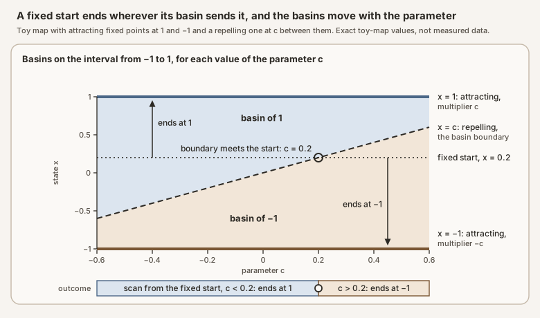
Scroll horizontally to inspect the diagram. The caption below provides a full text explanation.
Worked example
Take the map of one variable
\[ f_c(x)=x-\tfrac{1}{2}\,(x-c)\left(x^{2}-1\right), \]with a parameter \(c\) strictly between \(-1\) and \(1\). Its fixed points are \(-1\), \(c\), and \(1\), where the product vanishes. Their multipliers, the values there of the derivative \(f_c'(x)=1-\tfrac{1}{2}\left(3x^{2}-2cx-1\right)\), are \(-c\), \(1+\tfrac{1}{2}(1-c^{2})\), and \(c\). So \(1\) and \(-1\) are attracting, and \(c\), whose multiplier exceeds 1, is repelling. Near \(c\), the step \(f_c(x)-x=-\tfrac{1}{2}(x-c)(x^{2}-1)\) has the sign of \(x-c\), so states just above \(c\) move up and states just below it move down. For the values of \(c\) drawn below, from \(-0.6\) to \(0.6\), every start tested on the interval from \(-1\) to \(1\) ended at \(1\) if it lay above \(c\) and at \(-1\) if it lay below (4001 evenly spaced starts at each of 121 values of \(c\); a second run, with 199 values of \(c\) from \(-0.99\) to \(0.99\), agreed). On that interval, the repelling point is the boundary between the two basins, the one-dimensional counterpart of a saddle’s stable manifold.
Now fix the start at \(x_0=0.2\) and scan \(c\). For \(c=0\) the iterates are \(0.2\), \(0.296\), \(0.431033\), \(0.606509\), and so on, converging to \(1\). For \(c=0.4\) they are \(0.2\), \(0.104\), \(-0.042399\), \(-0.263201\), and so on, converging to \(-1\). The outcome jumps at \(c=0.2\), where the boundary passes through the start. Nothing bifurcates there: the multipliers of the three fixed points are \(-0.2\), \(1.48\), and \(0.2\), none on the unit circle, and both attractors exist on both sides of the jump.
Near the jump, the outcome takes longer to appear. At \(c=0.2\), a start \(10^{-6}\) above the boundary needs 30 steps to get 0.1 away from it, and a start \(10^{-9}\) above needs 48: about \(\ln 1000/\ln 1.48\approx17.6\) more steps for every factor of 1000 closer, the lingering rule of the stable manifold page with \(\mu_u=1.48\).
def endpoint(x0, c, max_steps=10_000, tol=1e-12):
    """Attractor reached from x0 under x -> x - (x - c)(x*x - 1)/2.

    Returns 1.0 or -1.0, or None if neither is within tol after max_steps.
    """
    if not -1.0 < c < 1.0:
        raise ValueError("c must lie strictly between -1 and 1")
    if not -1.0 <= x0 <= 1.0:
        raise ValueError("this example covers starts from -1 to 1")
    x = x0
    for _ in range(max_steps + 1):
        if abs(x - 1.0) <= tol:
            return 1.0
        if abs(x + 1.0) <= tol:
            return -1.0
        x = x - 0.5 * (x - c) * (x * x - 1.0)
    return None
[endpoint(0.2, c) for c in (-0.4, 0.0, 0.2, 0.4)] returns [1.0, 1.0, None, -1.0]. At \(c=0.2\) the start is the repelling fixed point itself and never moves, so it reaches neither attractor.
A basin is a property of the map, not of a single run: one trajectory shows only which basin holds its start, not how large the basin is or what shape it has. The share of random starts that end on an attractor measures the size of its basin only relative to the way the starts were drawn. And every start in a basin converges, but not necessarily quickly: near a boundary the transient can be long, as above.
The note on chaos in a language model’s feedback loop makes its parameter maps from one fixed start per cell, so where attractors coexist, a map shows the attractor whose basin holds that start. The note uses this to tell edges made by basin boundaries in its maps from bifurcation curves; the evidence is in the note.
See also: stable manifold, monodromy, Lyapunov exponent.