Stable manifold

The stable manifold of a fixed point or periodic orbit of a map is the set of states whose trajectories converge to it. Strictly, that whole set is the global stable set; the word manifold describes its shape near the point, as explained below. It matters most for a saddle, a point that attracts small deviations along some directions and repels them along others. A saddle’s stable manifold is a thin set: the states on it converge to the saddle, while almost every state near the saddle eventually leaves. Its counterpart, the unstable manifold, is made of the states that come out of the saddle: those whose past, traced back step by step, converges to it.

For a map \(F\), with \(x_{k+1}=F(x_k)\), and a fixed point \(p\), so that \(F(p)=p\), the stable manifold is

where \(F^{n}\) means \(n\) applications of \(F\). The unstable manifold \(W^u(p)\) is the set of states \(x\) that have a backward trajectory converging to \(p\): a sequence \(x_0=x, x_{-1}, x_{-2}, \ldots\) with \(F(x_{-k-1})=x_{-k}\) for every \(k\) and \(x_{-k}\to p\) as \(k\to\infty\). For a map that can be run backward, that sequence is simply the backward trajectory of \(x\). For a periodic orbit of period \(q\), the same definitions apply to each of its points with \(F^{q}\) in place of \(F\), and the orbit’s manifolds are the unions over its points.

Near \(p\), the derivative describes both sets. Let \(DF(p)\) be the Jacobian matrix of \(F\) at \(p\), or, for a periodic orbit, its monodromy matrix; its eigenvalues are the multipliers \(\mu\). The point is hyperbolic when no multiplier lies on the unit circle, \(\lvert\mu\rvert=1\). For a smooth map and a hyperbolic point, the stable manifold theorem says that the states whose trajectories stay near \(p\) and converge to it form a smooth surface through \(p\), the local stable manifold. It is tangent to the stable subspace, the directions that repeated application of \(DF(p)\) shrinks toward zero, and its dimension is the number of multipliers with \(\lvert\mu\rvert<1\), counted with multiplicity. The states with a backward trajectory that stays near \(p\) and converges to it likewise form the local unstable manifold, tangent to the directions that belong to the multipliers with \(\lvert\mu\rvert>1\). That local picture is what the word manifold refers to. Farther from \(p\), the global sets can bend and fold back, and they can return arbitrarily close to \(p\). Every state that \(F\) sends into the global stable set belongs to it as well, so for a map that is not invertible that set can have separate or branching pieces, and it need not be a manifold at all.

When exactly one multiplier lies outside the unit circle and none lies on it, the stable manifold has one dimension fewer than the state space: a curve in a plane, a surface in three dimensions, a hypersurface in general. Near the saddle it divides a small neighborhood into two sides. If that unstable multiplier \(\mu_u\) is positive, a deviation along the repelling direction keeps its sign, so states just on one side of the stable manifold leave along one branch of the unstable manifold, and states just on the other side leave along the other. When the two branches lead to different attractors, the stable manifold separates their basins of attraction.

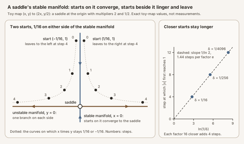
A state that starts a small distance \(\delta\) off the stable manifold first follows it toward the saddle and then leaves along the unstable manifold. When it arrives near the saddle, its component along the repelling direction is proportional to \(\delta\), and every period multiplies that component by \(\lvert\mu_u\rvert\). It therefore reaches a fixed size \(r\) after about

periods, where \(\ln\) is the natural logarithm. Each factor of \(e\approx2.718\), the base of the natural logarithm, by which \(\delta\) shrinks adds \(1/\ln\lvert\mu_u\rvert\) periods: the closer a start lies to the stable manifold, the longer it lingers near the saddle before it leaves.

Scroll horizontally to inspect the diagram. The caption below provides a full text explanation.

Worked example

Take the linear map of the plane

The origin is a saddle with multipliers 2, along \(x\), and \(1/2\), along \(y\). A state \((0,y)\) on the vertical axis goes to \((0, y/2^{n})\) after \(n\) steps and converges to the origin, so the vertical axis, \(x=0\), is the stable manifold. Any state with \(x\ne0\) has its \(\lvert x\rvert\) doubled on every step, so it eventually leaves. The horizontal axis, \(y=0\), is the unstable manifold, with one branch on each side of the origin.

Start at \((\delta, 1)\) with \(\delta=1/16\). The iterates are \((1/16, 1)\), \((1/8, 1/2)\), \((1/4, 1/4)\), \((1/2, 1/8)\), and \((1, 1/16)\). The product \(xy\) stays \(1/16\), so the state moves along a hyperbola. It comes closest to the saddle at step 2, at distance \(\sqrt{2}/4\approx0.354\), and reaches \(\lvert x\rvert=1\) at step 4. The start \((-1/16, 1)\), on the other side of the stable manifold, is the mirror image and leaves to the left.

A start 16 times closer, \(\delta=1/256\), reaches \(\lvert x\rvert=1\) at step 8 and comes within \(\sqrt{2}/16\approx0.088\) of the saddle; \(\delta=1/4096\) gives step 12 and \(\sqrt{2}/64\approx0.022\). Every factor of 16 adds 4 steps, that is, \(1/\ln 2\approx1.44\) steps per factor \(e\), the rule above with \(\mu_u=2\) and \(r=1\). The closest approach is \(\sqrt{2\delta}\), proportional to \(\delta^{1/2}\). More generally, take a linear saddle with one unstable direction and independent eigendirections, and a start whose stable component is of order one. The shrinking and the growing components balance near the closest approach, which is proportional to \(\delta^{\chi_s/(\chi_s+\chi_u)}\) up to a bounded factor from the whole-step timing, with \(\chi_u=\ln\lvert\mu_u\rvert\) and \(\chi_s=-\ln\lvert\mu_s\rvert\). Here \(\mu_s\) is the stable multiplier of largest modulus among the directions in which the start has a component; a start with no component along the slowest stable direction is governed by a faster one. In the example, \(\chi_s=\chi_u=\ln 2\), and the exponent is \(1/2\).

from math import hypot, isfinite


def passage(delta, radius=1.0, max_steps=10_000):
    """Follow (x, y) -> (2x, y/2) from (delta, 1).

    Returns the first step at which |x| >= radius (None if that does not happen
    within max_steps) and the smallest distance to the saddle up to that step.
    """
    if not isfinite(delta):
        raise ValueError("delta must be finite")
    if not isfinite(radius) or radius <= 0:
        raise ValueError("radius must be finite and positive")
    x, y = delta, 1.0
    closest = hypot(x, y)
    for step in range(max_steps + 1):
        if abs(x) >= radius:
            return step, closest
        x, y = 2.0 * x, 0.5 * y
        closest = min(closest, hypot(x, y))
    return None, closest

passage(1/16) returns (4, 0.3535...), passage(1/256) returns (8, 0.0883...), and passage(-1/16) also leaves at step 4, on the other side. passage(0.0) never leaves: its exit step is None, because a start exactly on the stable manifold converges to the saddle.

“Stable” describes the states on the manifold, not whether the manifold attracts its neighbors: near a saddle, states off the stable manifold leave. For an attracting point, with every multiplier inside the unit circle, the global stable set is the point’s whole basin of attraction, which contains a neighborhood of the point and so has as many dimensions as the state space.

In floating-point arithmetic a start exactly on a saddle’s stable manifold is generally out of reach. Rounding puts it on one side or the other, so even a start located by bisection to the last digit lingers near the saddle and then leaves, and how long it lingers measures how close it started. The estimates above are exact for the linear map. Near a nonlinear saddle, for small \(\delta\), the passage time still grows by \(1/\ln\lvert\mu_u\rvert\) periods per factor \(e\), up to an offset and the rounding to whole steps; the closest-approach exponent above is a prediction from the linearization.

The note on chaos in a language model’s feedback loop uses both manifolds: the unstable manifold of a period-3 saddle to describe a band of a chaotic attractor, and the stable manifold of a period-6 saddle orbit to explain an edge in its parameter maps, where it tests the passage-time rule above. The evidence for those conclusions is in the note.

See also: basin of attraction, monodromy, Lyapunov exponent.