Knowledge Base / Glossary
Forward-mode automatic differentiation
A way to compute a program's derivative along one input direction by carrying a tangent beside every value in a single forward pass.
Forward-mode automatic differentiation computes the derivative of a computer program along one chosen direction of its input. It runs the program once and carries, beside every intermediate number, a second number called its tangent: how fast that number changes as the input moves along the chosen direction. Each elementary operation updates the tangent by the chain rule, so when the program finishes, the tangents of its outputs are the derivative. There is no step size to choose and no truncation error; the result carries only the rounding error of its own arithmetic, like the value it accompanies.
Definition
Let a program compute a function \(f:\mathbb{R}^n\to\mathbb{R}^m\), from \(n\) input numbers to \(m\) output numbers, and assume that \(f\) is differentiable at the input \(x\): near \(x\) it is well approximated by a linear map. Its Jacobian \(J_f(x)\) is the \(m\times n\) matrix of that linear map. The entry in row \(i\) and column \(j\) is the partial derivative \(\partial f_i/\partial x_j\), the rate at which output \(i\) changes when only input \(j\) moves. For a direction \(v\in\mathbb{R}^n\), the Jacobian-vector product, often abbreviated JVP, is the rate at which all the outputs change as the input moves from \(x\) along \(v\), with \(h\) a scalar step that shrinks to zero:
\[ J_f(x)\,v=\lim_{h\to 0}\frac{f(x+hv)-f(x)}{h}. \]The program evaluates \(f\) as a sequence of elementary operations, each producing an intermediate value \(w_k\) from earlier ones. Forward mode gives the inputs the values \(x\) and the tangents \(v\), called the seed. For each operation \(w_k=\varphi_k(w_i, w_j)\) of two earlier values, it computes the value and, by the chain rule, the tangent:
\[ \dot w_k=\frac{\partial \varphi_k}{\partial w_i}\,\dot w_i+\frac{\partial \varphi_k}{\partial w_j}\,\dot w_j . \]A dot marks a tangent. When the program finishes, the tangents of the outputs are \(J_f(x)\,v\). The rules for the common elementary operations are short:
| Operation | Value | Tangent |
|---|---|---|
| sum | \(u+w\) | \(\dot u+\dot w\) |
| product | \(uw\) | \(\dot u\,w+u\,\dot w\) |
| quotient | \(u/w\) | \((\dot u\,w-u\,\dot w)/w^2\) |
| exponential | \(e^{u}\) | \(e^{u}\,\dot u\) |
| natural logarithm | \(\ln u\) | \(\dot u/u\) |
| sine | \(\sin u\) | \(\cos u\,\dot u\) |
These rules hold where the operations are differentiable: the quotient needs \(w\neq 0\), and the real logarithm needs \(u>0\).
The same bookkeeping is the arithmetic of dual numbers, numbers \(a+b\,\varepsilon\) with a formal symbol \(\varepsilon\) that satisfies \(\varepsilon^2=0\). Their product, \((a+b\,\varepsilon)(c+d\,\varepsilon)=ac+(ad+bc)\,\varepsilon\), is the product rule, and extending each elementary function \(g\) that is differentiable at \(a\) by \(g(a+b\,\varepsilon)=g(a)+g'(a)\,b\,\varepsilon\) reproduces the table. Evaluating the program on \(x+v\,\varepsilon\) then returns \(f(x)+J_f(x)\,v\,\varepsilon\).
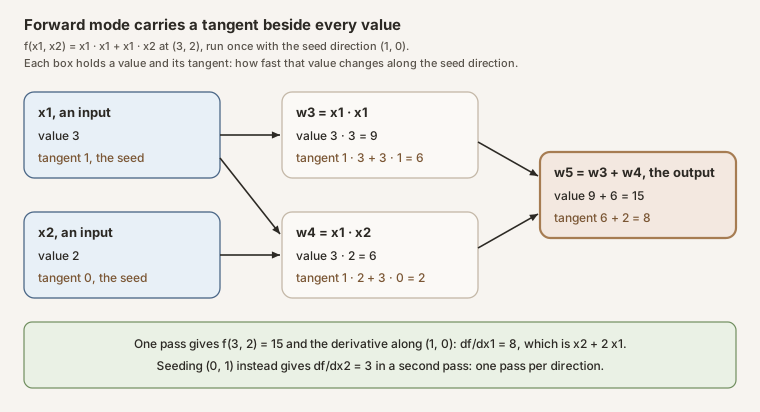
Scroll horizontally to inspect the diagram. The caption below provides a full text explanation.
Worked example
Let \(f(x_1,x_2)=x_1x_1+x_1x_2\) at \(x=(3,2)\), and seed the direction \(v=(1,0)\), which asks for \(\partial f/\partial x_1\). The inputs start with the tangents \(\dot x_1=1\) and \(\dot x_2=0\). The program runs three operations, and each value is computed together with its tangent. The values are
\[ \begin{aligned} w_3 &= x_1x_1 = 9,\\ w_4 &= x_1x_2 = 6,\\ w_5 &= w_3+w_4 = 15, \end{aligned} \]and the product and sum rules give the tangents
\[ \begin{aligned} \dot w_3 &= \dot x_1\,x_1+x_1\,\dot x_1 = 1\cdot 3+3\cdot 1 = 6,\\ \dot w_4 &= \dot x_1\,x_2+x_1\,\dot x_2 = 1\cdot 2+3\cdot 0 = 2,\\ \dot w_5 &= \dot w_3+\dot w_4 = 6+2 = 8. \end{aligned} \]So \(f(3,2)=15\) and \(\partial f/\partial x_1=8\), which agrees with the formula \(2x_1+x_2\). A second pass seeded with \(v=(0,1)\) gives \(\dot w_5=0+3=3=\partial f/\partial x_2=x_1\). Seeding \(v=(1,1)\) gives \(11=8+3\): the tangent is linear in the seed, as a Jacobian-vector product must be.
The minimal implementation below handles functions with one scalar output built from addition, multiplication and the supplied exp.
from dataclasses import dataclass
from math import exp as _exp


@dataclass(frozen=True)
class Dual:
    """A value and its tangent: the derivative along the chosen direction."""

    value: float
    tangent: float = 0.0

    def __add__(self, other):
        other = other if isinstance(other, Dual) else Dual(other)
        return Dual(self.value + other.value, self.tangent + other.tangent)

    def __mul__(self, other):
        other = other if isinstance(other, Dual) else Dual(other)
        return Dual(self.value * other.value,
                    self.tangent * other.value + self.value * other.tangent)

    __radd__ = __add__
    __rmul__ = __mul__


def exp(u):
    e = _exp(u.value)
    return Dual(e, e * u.tangent)


def jvp(f, point, direction):
    """For scalar-output f: its value at point and its derivative along direction."""
    out = f(*(Dual(p, d) for p, d in zip(point, direction, strict=True)))
    if not isinstance(out, Dual):
        raise TypeError("this toy jvp expects one Dual scalar output")
    return out.value, out.tangent


def f(x1, x2):
    return x1 * x1 + x1 * x2


print(jvp(f, (3.0, 2.0), (1.0, 0.0)))                # (15.0, 8.0)
print(jvp(f, (3.0, 2.0), (0.0, 1.0)))                # (15.0, 3.0)
print(jvp(lambda a: exp(a * a), (1.0,), (1.0,)))     # (2.718281828459045, 5.43656365691809)
The last line differentiates \(e^{a^2}\) at \(a=1\): the tangent \(2a\,e^{a^2}=2e\) comes out of the product rule and the exponential rule without any formula for the derivative being written down. Libraries provide the same operation for whole programs, for example jax.jvp in JAX and torch.func.jvp in PyTorch.
Cost, and the other mode
One forward pass costs a small constant multiple of one evaluation of the program, whatever the number of inputs, and gives one Jacobian-vector product: one combination of the columns of \(J_f(x)\). The full \(m\times n\) Jacobian takes \(n\) passes, one seed per input direction. Forward mode therefore suits functions with few inputs, or computations that need the derivative along only a few directions.
Reverse mode is the form of automatic differentiation used by backpropagation to train neural networks. It runs the program forward, then propagates sensitivities backward from the outputs. Given a weighting of the outputs \(u\in\mathbb{R}^m\), one backward pass gives the vector-Jacobian product \(u^{\top}J_f(x)\in\mathbb{R}^n\), where \(u^{\top}\) is \(u\) written as a row (its transpose): one weighted combination of the rows of the Jacobian. For a function with one output, such as a training loss, \(u=1\) gives the gradient, the vector of partial derivatives with respect to every input, after one forward and one backward pass, however many inputs there are. The price is memory: the backward pass needs the intermediate values of the forward pass, stored or recomputed.
A finite difference estimates the same Jacobian-vector product from two evaluations, \((f(x+hv)-f(x-hv))/(2h)\). For a sufficiently smooth function, the truncation error of this central formula shrinks like \(h^2\), because the function is not straight over the step. Subtracting two nearly equal outputs in floating point adds a rounding error that typically grows in proportion to \(1/h\), with a scale that depends on the problem, so the best step balances the two. Forward mode has no step to choose, no truncation error and no cancellation between nearby evaluations, because each tangent comes from the exact derivative rule of its operation. Its values and tangents are still rounded like any floating-point computation, and an inaccurate primitive operation passes its error on to them.
In these notes
The note on chaos in a language model’s feedback loop studies the soft-token map, which feeds a language model the probability-weighted average of its own token embeddings; its state has 896 coordinates. The note uses forward mode wherever it needs the derivative of that map along a few directions:
- To check the formula it derives for the map’s derivative. The note reports that along eight random directions, in float64 arithmetic, the formula and forward mode agree to a relative error of at most \(1.35\times10^{-13}\), while the best central differences reach only \(1.7\times10^{-9}\) to \(4.8\times10^{-9}\).
- To carry a tangent vector for Lyapunov exponents, the average rates at which nearby states separate. The note reports that at 448 randomly chosen settings of steering strength and temperature, the exponents from the forward-mode tangent and from twin trajectories, second runs started a tiny distance from the first, differ by at most 0.0041 nats per step, with a median difference of 0.0004.
- For Newton’s method on periodic orbits, which solves the orbit equation by repeated linearization, and for iterative eigenvalue and linear solvers that need only Jacobian-vector products. Chained along an orbit, those products stand in for the monodromy matrix, the derivative of one trip around the orbit, without forming it.
What it does not do
Forward mode differentiates the program as written, not the mathematical function the program is meant to compute. Where the program branches, it returns the derivative of the branch that ran: at a point where an absolute value or a rectified linear unit switches, or where the router of a mixture-of-experts model, which sends each token to its highest-scoring expert subnetworks, changes its choice, the result is a one-sided derivative or a library convention, not evidence that the function is smooth there. An approximation inside the program, such as a truncated series or a lookup table, is differentiated as the approximation it is. The tangents are computed in the program’s floating-point precision, so rounding still matters, and it can accumulate or be amplified when Jacobian-vector products are composed: a low-precision derivative of many steps can differ materially from a high-precision one even when each step looks accurate. The note reports such a case. A single Jacobian-vector product of one step in 32-bit floating point (float32) agrees with its 64-bit (float64) value to about \(5\times10^{-5}\), relatively, but the float32 derivative of eight composed steps differs from the float64 one by about 3%. Nor is forward mode symbolic differentiation: it returns numbers for one input and one direction, not a formula for the derivative.
An early description of forward accumulation is Wengert (1964), A simple automatic derivative evaluation program, Communications of the ACM 7(8), 463–464. Griewank and Walther (2008), Evaluating Derivatives: Principles and Techniques of Algorithmic Differentiation, second edition, SIAM, covers both modes and their costs.
See also: Lyapunov exponent, monodromy, covariance matrix.