Covariance matrix

A covariance matrix describes the shape of the cloud of values a random vector can take: how far the vector typically strays from its mean, and in which directions. For a random vector \(X\) with \(d\) coordinates it is a \(d \times d\) table, written \(\mathrm{Cov}(X)\). Each diagonal entry is the variance of one coordinate on its own, the square of its standard deviation. Each off-diagonal entry is the covariance of two coordinates: positive when they tend to stray from their means in the same direction, negative when they tend to stray in opposite directions, and zero when their paired deviations cancel on average. The one matrix answers the question for every direction at once. Take a direction given by a unit column vector \(w\), one with \(w^{\top}w = 1\), where the transpose \(w^{\top}\) is the same numbers written as a row. The coordinate of the random vector along that direction is the number \(w^{\top}X\), and its variance is \(w^{\top}\mathrm{Cov}(X)\,w\).

In these notes the covariance matrix matters for a reason beyond statistics. Suppose the weights of an average come from a softmax, as next-token probabilities do, and the scores behind the weights are computed from the same vectors that are averaged, as in a language model whose output layer reuses its input embeddings. Then the covariance matrix of those vectors is exactly how strongly the average responds to a change of the vector that produces the scores. In the soft-token loop that average is the soft token, the probability-weighted average of the token embeddings. The covariance of the embeddings under the model’s own next-token distribution therefore decides how strongly the readout of one step of the loop can amplify a small difference. It can be large only when tokens whose embeddings lie far apart share the probability, and it shrinks toward zero as one token takes nearly all of it.

Definition

A random vector \(X\) is a column of \(d\) coordinates, each of them a random number:

Write \(\mathbb{E}[\,\cdot\,]\), the expected value, for the probability-weighted average over the distribution of \(X\), and \(\mu = \mathbb{E}[X]\) for the mean. When every coordinate has a finite second moment, \(\mathbb{E}[X_i^2] < \infty\), the covariance matrix exists and is the expected outer product of the deviation from the mean:

It lines up with the coordinates one by one:

Row \(i\) and column \(j\) belong to the coordinates \(X_i\) and \(X_j\). The diagonal pairs each coordinate with itself, which gives its variance, and the matrix is symmetric because \(\mathrm{Cov}(X_i, X_j) = \mathrm{Cov}(X_j, X_i)\).

The rest of this entry needs only the finite case. Let \(X\) take the value \(v_k \in \mathbb{R}^d\) with probability \(p_k\), for \(k = 1, \dots, n\), where every \(p_k \ge 0\) and the \(p_k\) sum to 1. The expected values become probability-weighted sums. The mean of \(X\) is

and its covariance matrix is the probability-weighted average of the outer products of the deviations from that mean:

Here \(v_k - \mu\) is a column vector, and the outer product \((v_k - \mu)(v_k - \mu)^{\top}\) is the \(d \times d\) matrix whose entry in row \(i\) and column \(j\) is \((v_{k,i} - \mu_i)(v_{k,j} - \mu_j)\), the product of the deviations of coordinates \(i\) and \(j\), where \(v_{k,i}\) is coordinate \(i\) of \(v_k\). Entry by entry, then, \(\mathrm{Cov}(X_i, X_j) = \sum_k p_k\,(v_{k,i} - \mu_i)(v_{k,j} - \mu_j)\). On the diagonal, where \(j = i\), the product is a square, which is why the diagonal holds the variances. Multiplying out the product gives an equivalent form, the average of the outer products minus the outer product of the average:

When the source of the randomness needs saying, it goes in a subscript. In the soft-token notes, \(\mathrm{Cov}_{t\sim p}(e_t)\) means: draw a token \(t\) from the next-token distribution \(p\), and take its embedding \(e_t\) as the random vector. The mean of that draw, \(\sum_t p_t e_t\), is the soft token, a point of the convex hull of the embeddings. If the vectors \(v_k\) are stacked as the rows of an \(n \times d\) matrix \(E\), not to be confused with the expected value \(\mathbb{E}\), the same covariance matrix is

where \(\mathrm{diag}\,p\) is the \(n \times n\) diagonal matrix with \(p_1, \dots, p_n\) on its diagonal. The two pieces match the two terms above: \(E^{\top}(\mathrm{diag}\,p)E = \sum_k p_k\,v_k v_k^{\top}\) and \(E^{\top}pp^{\top}E = \mu\mu^{\top}\).

Scroll horizontally to inspect the diagram. The caption below provides a full text explanation.

Worked example

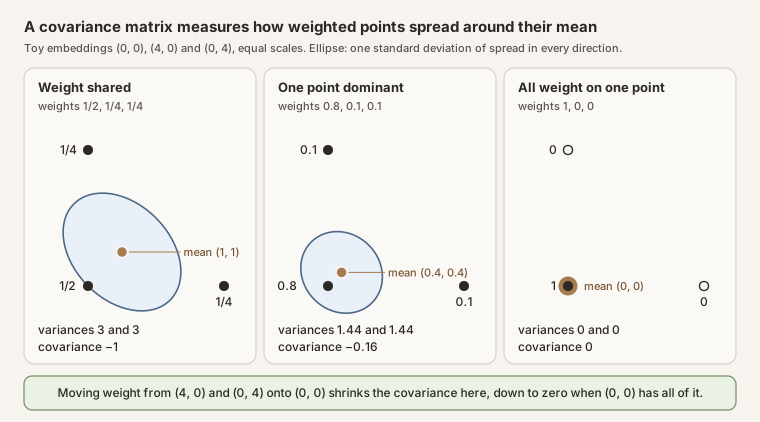
Let \(X = (X_1, X_2)\) be the random vector that equals one of the toy embeddings \(v_1 = (0, 0)\), \(v_2 = (4, 0)\) and \(v_3 = (0, 4)\), with probabilities \(1/2\), \(1/4\) and \(1/4\). The mean is

and the deviations from it are \((-1, -1)\), \((3, -1)\) and \((-1, 3)\). Weighting their outer products by the probabilities and adding gives

So \(\mathrm{Var}(X_1) = \mathrm{Var}(X_2) = 3\): both coordinates have variance 3. Their covariance, \(\mathrm{Cov}(X_1, X_2) = -1\), is negative because the draws that land right of the mean, at \((4, 0)\), land below it. The second form agrees: \(\sum_k p_k\,v_k v_k^{\top}\) has 4 in both diagonal entries and 0 elsewhere, and \(\mu\mu^{\top}\) has 1 in every entry.

The spread also depends on direction. Along \(w = (1, -1)/\sqrt{2}\), the line from \((0, 4)\) to \((4, 0)\), the variance \(w^{\top}\mathrm{Cov}(X)\,w\) is 4; along the perpendicular direction \((1, 1)/\sqrt{2}\) it is 2. These two directions are the eigenvectors of the matrix, and 4 and 2 are its eigenvalues. They are the axes of the ellipse in the figure, whose half-lengths are the square roots, 2 and \(\sqrt{2}\).

In this example, moving weight onto \((0, 0)\) shrinks the matrix. With probabilities \(0.8\), \(0.1\) and \(0.1\), the mean is \((0.4, 0.4)\), \(\sum_k p_k\,v_k v_k^{\top}\) has 1.6 in both diagonal entries and 0 elsewhere, and \(\mu\mu^{\top}\) has 0.16 in every entry. With all the weight on \((0, 0)\), the mean is that point and every deviation is zero. The two covariance matrices are

Why a softmax average responds with its covariance

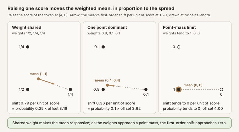
Suppose the weights of the average are a softmax of scores \(z_t\) at temperature \(T\), so that \(p = \mathrm{softmax}(z/T)\) and the mean is \(\mu = \sum_t p_t e_t\). Raise one score, \(z_k\), by a small amount \(\delta\). The softmax raises that token’s probability by \(\tfrac{\delta}{T}\,p_k(1 - p_k)\) and lowers every other probability \(p_t\) by \(\tfrac{\delta}{T}\,p_t p_k\). Adding up the weighted embeddings, the mean moves by

The mean moves toward the token whose score rose, by an amount proportional to that token’s probability and to its distance from the mean. A token with almost no probability barely moves it, and neither does a token that already sits at the mean.

Now let the scores come from a hidden vector \(h\), \(z_t = e_t^{\top}h\), as they do in a model whose output layer reuses its input embeddings. A small push \(w\) of \(h\) raises every score at once, \(z_t\) by \(e_t^{\top}w\). Adding up the moves for all tokens gives

The last step subtracts \(\mu\) inside \(e_t^{\top}w\), which changes nothing because the weighted deviations \(p_t(e_t - \mu)\) add up to zero. So the covariance matrix, divided by \(T\), is the derivative of the softmax average with respect to the hidden vector. The average moves far in the directions where the embeddings spread under \(p\), and not at all in the directions where they do not.

For finite scores and \(T > 0\), every softmax probability is positive: a softmax never puts all the weight on one token, it only approaches that as one score comes to dominate. The right-hand panel below is that limit.

Scroll horizontally to inspect the diagram. The caption below provides a full text explanation.

In the worked example, take \(T = 1\) and the scores \((0, -\ln 2, -\ln 2)\), whose softmax is the weights \(1/2\), \(1/4\) and \(1/4\). Raising the score of \((4, 0)\) by \(\delta = 0.1\) should move the mean by about \(0.1 \times \tfrac14 \times (3, -1) = (0.075, -0.025)\). Recomputing the softmax exactly gives the weights 0.4872, 0.2692 and 0.2436 and moves the mean by \((0.0769, -0.0256)\), the first-order prediction up to a term of order \(\delta^2\). The same scores come from the hidden vector \(h = (-\ln 2/4, -\ln 2/4)\) through \(z_t = e_t^{\top}h\). A push \(w = (0.1, 0)\) of \(h\) raises only the score of \((4, 0)\), by 0.4, and moves the mean by \(\mathrm{Cov}(X)\,w = (0.3, -0.1)\) to first order: four times the move above.

This is the readout half of the soft-token loop’s derivative. There the hidden vector is the network’s final state, the averaged vectors are the token embeddings, and the mean is the next soft token. One step of the loop turns a small change \(dx\) of the input into the change \(\mathrm{Cov}_{t\sim p}(e_t)\,J\,dx/T\) of the next soft token, where \(J\) is the derivative of the network’s final state with respect to its input. The two parts of the readout pull against each other at low temperature: \(1/T\) grows, but if one score is strictly the highest, \(p\) concentrates on that token as \(T\) falls and the covariance tends to zero. If several scores tie for the top, the probability stays split among them and the covariance need not vanish. Large amplification needs both at once: probability shared among tokens whose embeddings lie far apart, and a temperature low enough to magnify that spread, along the directions that the network’s derivative \(J\) feeds.

from math import exp, log


def weighted_covariance(points, weights):
    """Covariance matrix of a random vector that equals points[k] with probability weights[k]."""
    if len(points) == 0 or len(points) != len(weights):
        raise ValueError("points and weights must be nonempty and the same length")
    if any(weight < 0 for weight in weights):
        raise ValueError("weights must be nonnegative")
    if abs(sum(weights) - 1.0) > 1e-12:
        raise ValueError("weights must sum to one")
    d = len(points[0])
    if any(len(point) != d for point in points):
        raise ValueError("points must all have the same length")
    mean = [sum(w * point[i] for w, point in zip(weights, points)) for i in range(d)]
    return [
        [
            sum(w * (point[i] - mean[i]) * (point[j] - mean[j]) for w, point in zip(weights, points))
            for j in range(d)
        ]
        for i in range(d)
    ]


def softmax_mean(points, scores, temperature=1.0):
    """Softmax weights of the scores and the weighted mean of the points."""
    top = max(scores)
    weights = [exp((s - top) / temperature) for s in scores]
    total = sum(weights)
    probs = [w / total for w in weights]
    mean = [sum(p * point[i] for p, point in zip(probs, points)) for i in range(len(points[0]))]
    return mean, probs


points = [(0.0, 0.0), (4.0, 0.0), (0.0, 4.0)]


def scores_at(h):
    return [sum(e * x for e, x in zip(point, h)) for point in points]


h = (-log(2) / 4, -log(2) / 4)
mean, probs = softmax_mean(points, scores_at(h))           # weights 1/2, 1/4, 1/4
cov = weighted_covariance(points, probs)                   # [[3, -1], [-1, 3]]
step = 1e-6
moved, _ = softmax_mean(points, scores_at((h[0] + step, h[1])))
print([round((m - m0) / step, 4) for m, m0 in zip(moved, mean)])   # [3.0, -1.0]
print([round(row[0], 12) for row in cov])                          # [3.0, -1.0], Cov times (1, 0)

The two printed lines agree: pushing \(h\) along \((1, 0)\) moves the mean along the first column of the covariance matrix.

Properties

• Symmetric. The entry in row \(i\) and column \(j\) equals the entry in row \(j\) and column \(i\).
• Never negative in any direction. For every vector \(w\), \(w^{\top}\mathrm{Cov}(X)\,w\) is the variance of \(w^{\top}X\), so it is at least 0. The matrix is therefore positive semidefinite, and its eigenvalues are nonnegative. Its leading eigenvector is the direction of largest spread, which is what principal component analysis uses.
• Zero exactly when there is no spread. The matrix is zero if and only if all the points with positive probability coincide, for example when one point has all the probability. A softmax average with a zero covariance cannot be moved by any small change of its scores.
• Low rank when few points share the weight. The weighted deviations \(p_k(v_k - \mu)\) sum to zero, so with \(m\) points of positive probability the matrix has rank at most \(m - 1\). With two points it is \(p_1 p_2\,(v_1 - v_2)(v_1 - v_2)^{\top}\), of rank one: a softmax average of two vectors can move only along the line between them, fastest when \(p_1 = p_2 = 1/2\).
• Units. If \(X_i\) is measured in the unit \(U_i\), then \(\mathrm{Var}(X_i)\) carries \(U_i^2\) and \(\mathrm{Cov}(X_i, X_j)\) carries \(U_i U_j\), so the entries change with the scale of the coordinates. Directions and eigenvectors are meaningful only when the coordinates share a unit, as embedding coordinates do, or have been scaled deliberately. Pearson correlation divides each covariance by the two standard deviations to remove the units.

Conventions

With \(n\) equally weighted observations, \(p_k = 1/n\), the definition gives the population covariance of those observations. To estimate the covariance of a larger population from \(n\) random draws, many programs divide by \(n - 1\) instead of \(n\), the same choice as for the standard deviation. The soft-token covariance involves no estimation: it is exact for the stated distribution.

For two random vectors drawn together, taking the values \(x_k\) and \(y_k\) with probability \(p_k\), the cross-covariance is \(\mathrm{Cov}(X, Y) = \sum_k p_k\,(x_k - \mu_X)(y_k - \mu_Y)^{\top}\), where \(\mu_X\) and \(\mu_Y\) are their means. It is not symmetric in general. It replaces the covariance in the derivative above when the scores come from different vectors than the ones averaged, \(z_t = w_t^{\top}h\): the mean then moves by \(\mathrm{Cov}_{t\sim p}(e_t, w_t)\,w/T\). In the soft-token notes this is the case of models whose output vectors \(w_t\) differ from their input embeddings \(e_t\).

What it does not show

A covariance matrix measures linear co-variation only. Zero covariance does not mean independence: if \(x\) is \(-1\), 0 or 1 with equal probability and \(y = x^2\), their covariance is 0 although \(y\) is a function of \(x\). A covariance says nothing about cause, and its entries change with the units of the coordinates. In the soft-token notes, \(\mathrm{Cov}_{t\sim p}(e_t)\) is a property of one next-token distribution at one state of the loop, not a statistic estimated from data. A large covariance makes the soft token easy to move, but whether the loop as a whole stretches small differences also depends on the network’s derivative \(J\).

See also: embedding, convex hull, logit, temperature, standard deviation, Pearson correlation, Lyapunov exponent.