Knowledge Base / Glossary
Pearson correlation
A number from negative one to positive one that summarizes the direction and strength of a linear relationship between two numerical features.
Pearson correlation, usually written \(r\), summarizes the direction and strength of a linear relationship between two numerical features. Its value ranges from \(-1\) to \(+1\).
- A value near \(+1\) means high values of one feature tend to accompany high values of the other in an almost straight-line pattern.
- A value near \(-1\) means high values of one tend to accompany low values of the other.
- A value near \(0\) means little straight-line relationship. A curved relationship can still be present.
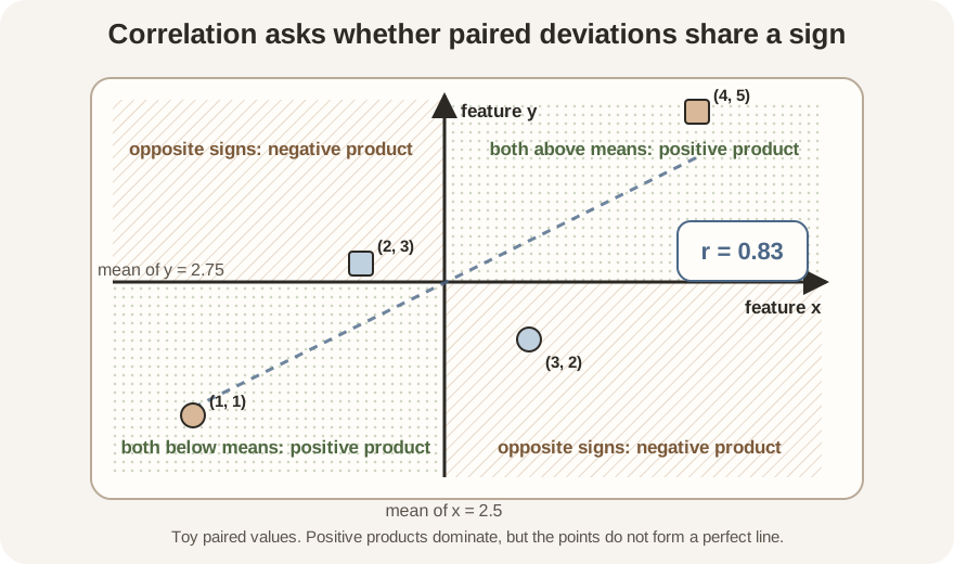
Scroll horizontally to inspect the diagram. The caption below provides a full text explanation.
The calculation
Suppose \(n\) observations each have a paired value \(x_i\) from feature \(x\) and \(y_i\) from feature \(y\). Let \(\bar{x}\) and \(\bar{y}\) be the two feature means. Pearson correlation is
\[ r= \frac{\sum_{i=1}^{n}(x_i-\bar{x})(y_i-\bar{y})} {\sqrt{\sum_{i=1}^{n}(x_i-\bar{x})^2} \sqrt{\sum_{i=1}^{n}(y_i-\bar{y})^2}}. \]The numerator adds products of paired deviations from the means. The denominator divides by the two features’ spread, making \(r\) independent of a simple change of positive scale such as millimeters to centimeters.
Worked example
Take four pairs:
| observation | \(x\) | \(y\) |
|---|---|---|
| 1 | 1 | 1 |
| 2 | 2 | 3 |
| 3 | 3 | 2 |
| 4 | 4 | 5 |
The means are \(\bar{x}=2.5\) and \(\bar{y}=2.75\). The numerator is \(5.5\), the two sums of squared deviations are \(5\) and \(8.75\), and therefore
\[ r=\frac{5.5}{\sqrt{5\times8.75}}\approx0.83. \]The pairs show a fairly strong positive linear tendency, but they do not sit perfectly on one line. These four values are a calculation example, not enough evidence for a biological population claim.
Important boundaries
- Correlation requires paired measurements on the same observations. Shuffling one feature’s rows changes the question and usually changes \(r\).
- If either feature is constant, its spread is zero and \(r\) is undefined.
- One extreme observation can have a large effect.
- A high absolute correlation does not prove that one feature causes the other. Both may respond to a third factor.
- A near-zero value does not rule out a curved association or group-specific relationships.
- A sample correlation is not automatically a precise population estimate. Dependence, sampling design, and uncertainty still matter.
In principal component analysis, a correlation matrix can reveal features that carry overlapping linear information. PCA can summarize that shared variation, but it does not turn correlation into causation.
See also: standard deviation, standard scaling, and principal component analysis.