Principal component analysis (PCA)

Principal component analysis (PCA) turns several numerical feature columns into a new set of coordinate axes. The first new axis follows the direction in which the observations are most spread out. That spread is variation; variance is one numerical way to measure it by averaging squared distances from the mean. Each later axis is perpendicular to the earlier axes and captures as much remaining variance as it can.

PCA is a form of dimensionality reduction. A table with seven feature columns has seven dimensions. Plotting only its first two principal components gives a two-dimensional summary. That summary is easier to inspect, but it can leave variation out. The explained-variance ratio reports how much of the dataset’s total variance the displayed components retain.

For a complete biological example with real wheat-kernel measurements, inline Python, and interpretation guidance, use the full PCA Deep Dive.

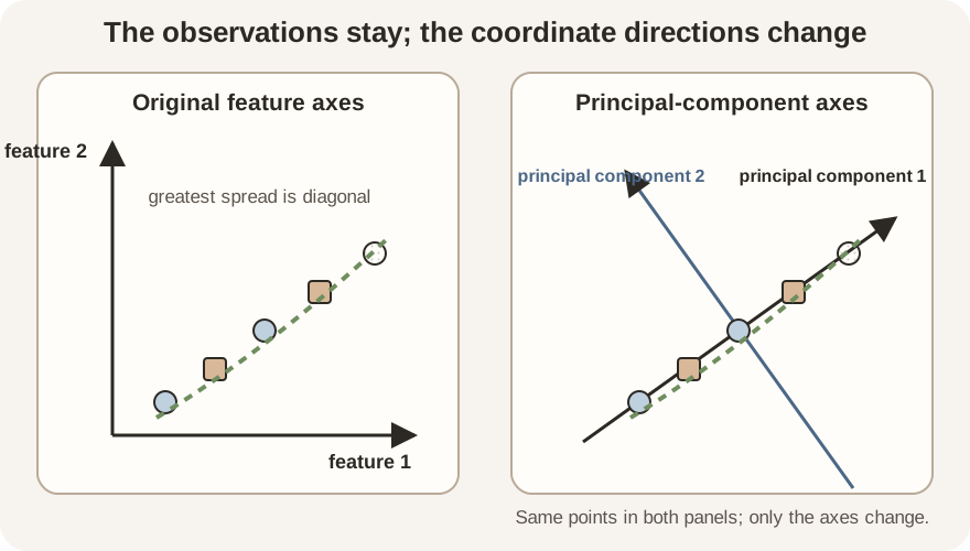
Scroll horizontally to inspect the diagram. The caption below provides a full text explanation.

What the calculation does

Think of a data table with one observation per row and one measurement per feature column. PCA then:

1. centers each feature by subtracting its mean;
2. optionally uses standard scaling when the scientific question calls for comparable feature scales;
3. finds a unit-length direction through feature space with the greatest variance;
4. projects every observation onto that direction to produce its first principal-component score; and
5. repeats the search for perpendicular directions that capture successively less of the remaining variance.

A score is one observation’s coordinate on a principal component. A principal-axis coefficient is the weight assigned to one original feature when constructing that component. Reading scores and coefficients together connects a point on the map back to the original measurements.

A two-feature score

Suppose a toy observation has standardized coordinates \(x=(1.25,0.50)\). Its first principal-axis direction is \(v=(0.80,0.60)\). The direction has length one because \(0.80^2+0.60^2=1\). The observation’s PC1 score is the weighted sum

\[ x\mathbin{\cdot}v =(1.25\times0.80)+(0.50\times0.60) =1.30. \]

The dot symbol means multiply matching coordinates and add the products. The numbers are a teaching example, not fitted coefficients from a dataset. In a real analysis, software learns the direction from all rows.

Choices that change the map

• Rows and features: adding or removing observations or feature columns changes the matrix PCA summarizes.
• Units and scaling: an unscaled feature with large numerical variance can dominate even when its units, rather than its biology, created that scale.
• Missing values: most PCA implementations require a complete matrix, so exclusions or imputation become part of the analysis.
• Displayed components: a two-component plot can hide differences that lie mainly in later components.
• Signs: multiplying one component’s coefficients and every corresponding score by \(-1\) mirrors the axis without changing the PCA result.

What PCA does not establish

• A cluster is not automatically a biological class or a statistically significant group difference.
• Separation does not show that a measured feature caused the separation.
• Explained variance is not prediction accuracy or the percentage of biology explained.
• A descriptive full-dataset PCA does not demonstrate performance on new observations. That requires a held-out evaluation protected from data leakage.

See also: standard deviation, standard scaling, and Pearson correlation.