Knowledge Base / Deep Dives
Late Chunking: Context Before Pooling
Late chunking lets an embedding model contextualize a longer input before pooling smaller retrieval chunks, preserving one vector per chunk without promising that more context always helps.
On this page 19 sections
Late chunking creates an embedding for each small retrieval chunk after a transformer has read a longer input containing that chunk. The chunk boundaries can stay exactly where they were. What moves later is the moment when those boundaries are used for pooling.
That distinction matters:
- Late chunking does not ask a model to choose the chunk boundaries.
- It does not store one vector for every token.
- It does not guarantee better retrieval whenever more context is available.
- It does require access to token-level states from a compatible embedding model.
The method was introduced by Günther et al. in Late Chunking: Contextual Chunk Embeddings Using Long-Context Embedding Models. This Deep Dive explains the operation, the published evidence, the implementation boundaries, and the cases where the standard approach can still win.
Choose a reading route.
- Learning the idea: continue with the vocabulary, short example, and step-by-step operation.
- Assessing the evidence: start with retrieval scoring, then the published evaluation and SciFact re-evaluation.
- Implementing or reproducing it: read the implementation boundary, evaluation plan, and reproduction appendix.
Before late chunking: a tiny vocabulary kit
- A token is one piece of text produced by tokenization. A token might be a word, part of a word, or punctuation.
- A contextual token state is the model’s list of numbers for one token after it has read the surrounding tokens allowed by its attention mask. The same word can therefore receive different numbers in different sentences.
- A vector is an ordered list of numbers. An embedding is a vector used to represent an item so that a retrieval system can compare it with other items.
- A retrieval chunk is one stored piece of a document that search may return.
- Mean pooling averages several token-state vectors coordinate by coordinate to make one chunk vector.
- L2 normalization rescales a nonzero vector to length 1. It does not choose chunk boundaries or add context.
These definitions are deliberately local and practical. The linked glossary entries give formulas, edge cases, and small diagrams when you want them.
The short version
Suppose a document contains three chunks:
- “Berlin is the capital and largest city of Germany.”
- “Its population exceeds 3.85 million.”
- “The city is also one of Germany’s states.”
With naive chunking, the embedding model encodes each numbered span independently. Tokens such as Its and The city cannot attend to the earlier mention of Berlin during that encoding pass.
With late chunking, the model encodes all three spans in one in-window input. It then mean-pools the token states inside each of the same three spans. Earlier context can influence the vectors for spans 2 and 3, but only tokens assigned to each span are pooled into that span’s final vector.
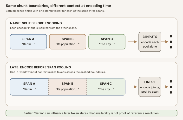
Scroll horizontally to inspect the diagram. The caption below provides a full text explanation.
The operation, one step at a time
For one document that fits the encoder’s usable window:
- Choose the retrieval chunks. Record exactly which text belongs to each chunk.
- Tokenize the longer input once. Keep the mapping from the original chunk boundaries to token positions.
- Run the transformer once. Retain one contextual state vector for every usable token position.
- Average within each chunk. For each recorded span, mean-pool only the token states assigned to that span.
- Normalize each chunk vector. Divide each nonzero mean vector by its L2 length if that is the embedding model’s documented recipe.
The result is still one vector per retrieval chunk. The difference is that each token state could use context from outside its final chunk before the averaging step.
A tiny runnable pooling example
The next cell starts after a transformer has produced four toy token states. It shows only averaging, masking, and L2 normalization. Paste it into a Colab or local Python cell with NumPy installed.
import numpy as np

# Four already-contextualized token states, each with two coordinates.
token_states = np.array([
    [1.0, 0.0],
    [1.0, 2.0],
    [3.0, 0.0],
    [99.0, 99.0],  # padding: the mask below excludes this row
])
attention_mask = np.array([1, 1, 1, 0], dtype=bool)
spans = [(0, 2), (2, 4)]  # half-open: start included, stop excluded

chunk_vectors = []
for start, stop in spans:
    usable_states = token_states[start:stop][attention_mask[start:stop]]
    mean_vector = usable_states.mean(axis=0)
    unit_vector = mean_vector / np.linalg.norm(mean_vector)
    chunk_vectors.append(unit_vector)

chunk_vectors = np.vstack(chunk_vectors)
print(np.round(chunk_vectors, 4))
print(np.round(np.linalg.norm(chunk_vectors, axis=1), 4))
Expected output:
[[0.7071 0.7071]
 [1.     0.    ]]
[1. 1.]
The first chunk averages \([1,0]\) and \([1,2]\) to get \([1,1]\), then rescales it to about \([0.7071,0.7071]\). The second span contains one usable state because the padding row is masked out. This small example teaches the mechanics, not how a real model creates the contextual states.
What changes and what stays fixed
| Property | Naive chunking | Late chunking |
|---|---|---|
| Chunk text and boundaries | Chosen before encoding | Chosen before encoding |
| Transformer input | One chunk at a time | A longer input containing several chunks |
| Pooling | Over states conditioned on that chunk | Over the same span’s states, conditioned on the longer input |
| Stored representation | One vector per chunk | One vector per chunk |
| Query encoding | Model’s documented query path | The same documented query path |
| Context reach | The isolated chunk | The encoder’s usable input window |
Late chunking changes the chunk vectors by changing the text available while the model creates token states. It does not change the model parameters or output dimensionality, and there is no per-document retraining.
A worked example, and its limit
The paper’s introductory Berlin example compares the query Berlin with three sentence embeddings produced by jina-embeddings-v2-small-en. Its reported cosine similarities are:
| Sentence | Naive | Late |
|---|---|---|
| Contains “Berlin” directly | 0.8486 | 0.8495 |
| Begins “Its more than 3.85 million inhabitants…” | 0.7084 | 0.8249 |
| Begins “The city is also one of the states…” | 0.7535 | 0.8498 |
This is a useful mechanism-level illustration: the two later sentence vectors change when their token states are conditioned on the preceding sentence. It is not a retrieval benchmark. A cosine increase for one query does not establish a better ranking, fewer false matches, or correct interpretation of every phrase that refers back to an earlier phrase. Those claims require a corpus, queries, relevance judgments, and retrieval metrics.
Source: Günther et al., Table 1.
How retrieval is scored
A retrieval benchmark supplies three connected ingredients:
- a query, such as a scientific claim that needs supporting evidence;
- a corpus, meaning the collection of documents that can be returned; and
- relevance judgments, often stored in a file called qrels, that record which query-document pairs count as relevant under the benchmark.
The search system ranks the corpus for each query. The notation @10 means that the metric inspects only the first ten returned documents.
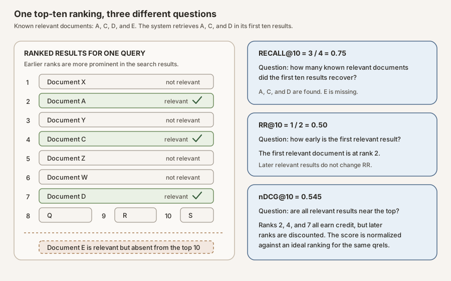
Scroll horizontally to inspect the diagram. The caption below provides a full text explanation.
What the published retrieval evaluation found
The paper compares naive and late chunking on four selected datasets from the Benchmarking Information Retrieval (BEIR) collection, NFCorpus, SciFact, FiQA, and TREC-COVID, using three embedding models. Each dataset supplies queries, a document corpus, and qrels that identify relevant documents. Chunk rankings are converted to document rankings under the paper’s protocol and scored with nDCG@10.
The paper reports nDCG@10 on a 0-100 scale. The changes below are absolute points on that reporting scale:
| Boundary method | Naive nDCG@10 (×100) | Late nDCG@10 (×100) | Paper-reported change (points) |
|---|---|---|---|
| Five sentences per chunk | 52.4 | 54.3 | +1.9 |
| 256 tokens per chunk | 52.2 | 54.0 | +1.8 |
| Semantic sentence boundaries | 52.4 | 53.8 | +1.5 from unrounded scores |
The displayed 52.4 and 53.8 values are rounded to one decimal place, while the reported +1.5 change was calculated from the unrounded values. That is why subtracting the displayed endpoints appears to give 1.4.
These are averages across the paper’s three models and four selected BEIR tasks, not expected gains for a new corpus. The evaluation used non-overlapping retrieval chunks and a specific protocol for assigning instruction and special-token states to the first or last chunk. See Section 4.1 for the table and Section 4.2 for the chunk-size ablation, meaning a comparison that deliberately changes chunk size while keeping the rest of the intended protocol fixed.
The aggregate hides heterogeneous results. In Section 4.2’s nDCG retrieval ablation, the authors use jina-embeddings-v2-small-en, fixed-size chunks at several tested sizes, NFCorpus and LongEmbed tasks, and truncate inputs at 8,192 tokens. They report stronger late-chunking results particularly at smaller chunk sizes, while some reading-comprehension configurations with larger chunks favor naive chunking. They also report no late-chunking benefit on the tested Needle-8192 and Passkey-8192 configurations, where short relevant text is placed inside unrelated context. Those are results and interpretations for that experiment, not a rule that a task family universally favors either method.
The defensible conclusion is that late chunking can improve retrieval when surrounding text helps represent the target span. “More context is always better” is not supported.
An auditable SciFact matched-content-token re-evaluation
This page also ships a runnable re-evaluation on the complete SciFact test candidate corpus: 5,183 documents, 300 test queries, and 339 positive query-document judgments. Under this benchmark protocol, query-document pairs absent from the qrels are treated as nonrelevant. The run uses jina-embeddings-v2-small-en at commit 44e7d1d, its remote implementation at commit f3ec4cf, and 256-content-token spans without overlap. The frozen corpus produced 9,356 chunks. Its longest document had 1,937 content tokens, so no document was truncated against the model’s 8,192-token limit.
The naive and late arms match many important choices, but not every model input. This is an end-to-end protocol comparison rather than a context-only causal test.
| Comparison question | Frozen answer |
|---|---|
| Held fixed | Corpus, queries, tokenizer and model revisions, content-token IDs and spans, query path, mean pooling, L2 normalization, and cosine scoring |
| Different by design | Every naive chunk gets its own [CLS] start token and [SEP] end token. The late arm uses one document-level pair, assigned to the first and last spans. Independently encoded chunks can also use different position-dependent inputs. |
| Measured | Full-corpus document nDCG@10, Recall@10, MRR@10, query-level changes, and descriptive query-bootstrap intervals |
| Not isolated | The effect of cross-span context by itself. Special tokens and position-dependent inputs can influence content-token states even when their own states are not included in the final mean. |
A stricter context-only ablation, meaning a test that changes one intended factor, would hold every non-contextual encoder input and every pooled position fixed, then vary only cross-span context or attention. Where a compatible model supports it, one possible design is to encode the same token sequence with carefully matched full-attention and block-diagonal attention masks. An ordinary padding attention mask merely marks usable positions; it does not automatically prevent one chunk from attending to another.
The three evaluated document representations are:
- Naive chunks: each frozen content-token slice receives its own special tokens and is encoded independently.
- Late chunks: the complete document is encoded once, then the same content-token spans are pooled.
[CLS]belongs to the first span and[SEP]to the last. - Whole document: the same full-document states used by the late arm are pooled into one vector. This is a control for “use all context” without retaining one retrieval vector per chunk.
Queries receive no instruction prefix and use the same attention-mask mean pooling and L2 normalization in every arm. The script scores every corpus chunk, takes each document’s maximum chunk score for the two chunked arms, ranks the complete document corpus, and calculates document-level nDCG@10, Recall@10, and MRR@10 from the frozen binary qrels. Stable corpus order breaks exact score ties.
This is an auditable matched-content-token re-evaluation, not an exact replication of one paper-table cell or a context-only causal ablation. The pinned paper helper decodes token slices before its evaluator retokenizes them; that can alter boundary tokenization. This version passes the original token IDs directly so the naive and late arms share exact content spans. It also scores the full corpus before max-chunk document aggregation instead of collapsing a previously retrieved candidate-chunk list. Those choices make the content-token comparison cleaner for this tutorial, but its values should not be substituted for the paper’s protocol.
The intervals below use a query bootstrap: repeatedly resample the 300 query rows with replacement, recompute the summary, and inspect how much it moves. These are descriptive stability intervals for the fixed benchmark, not population confidence intervals.
![SciFact test document nDCG at 10 on a zero-to-one axis, with query-bootstrap intervals: naive 256-token chunks 0.6414 [0.5942, 0.6876]; late 256-token chunks 0.6610 [0.6145, 0.7071]; whole-document encoding 0.6389 [0.5918, 0.6852]. Higher is better.](/blog/knowledge-base/deep-dives/late-chunking/fig-scifact-retrieval.svg)
Scroll horizontally to inspect the diagram. The caption below provides a full text explanation.
| Document representation | nDCG@10 | 95% query-bootstrap interval | Recall@10 | MRR@10 |
|---|---|---|---|---|
| Naive 256-token chunks | 0.6414 | [0.5942, 0.6876] | 0.7626 | 0.6123 |
| Late 256-token chunks | 0.6610 | [0.6145, 0.7071] | 0.7776 | 0.6337 |
| Whole document | 0.6389 | [0.5918, 0.6852] | 0.7592 | 0.6105 |
Late chunking had the highest aggregate score of these three arms, but the aggregate hides how sparse the changes were.
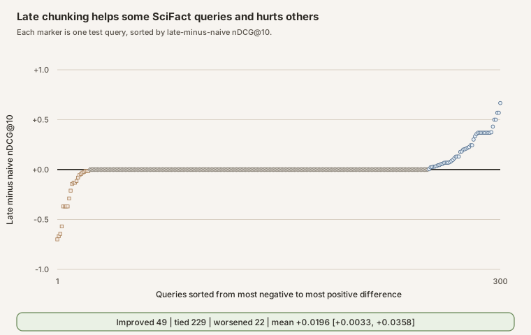
Scroll horizontally to inspect the diagram. The caption below provides a full text explanation.
| Paired comparison | Mean nDCG@10 difference | 95% paired query-bootstrap interval | Improved | Tied | Worsened |
|---|---|---|---|---|---|
| Late minus naive | +0.0196 | [+0.0033, +0.0358] | 49 | 229 | 22 |
What did this re-evaluation teach us?
The re-evaluation supports five conclusions:
- Late chunking had the highest mean ranking score in this comparison. Its nDCG@10 was 0.6610, compared with 0.6414 for naive chunks and 0.6389 for one whole-document vector.
- The gain was not shared evenly. Late chunking improved 49 queries, tied on 229, and worsened 22. The positive average did not mean every query benefited.
- The one-vector whole-document baseline scored lower, but it does not isolate why. Full-document context followed by one pooled vector scored below the late-chunk arm. The chunked arm stores several candidate vectors and uses maximum-score aggregation, so the difference can reflect representation granularity and aggregation as well as contextualization. This is a practical baseline, not a capacity-matched causal control.
- The comparison does not isolate context alone. The naive and late arms differ in their special-token and position-dependent inputs as well as in cross-chunk context.
- The practical answer is to test, not assume. A representative corpus can reveal whether the ranking improvement is large enough to justify the added indexing cost and memory.
The full audit trail and commands are in Appendix A.
The implementation boundary
Late chunking needs more than an application programming interface (API) that returns one already-pooled vector for an input. You need:
- token-level hidden states from the embedding model;
- one frozen tokenization of the longer input;
- one half-open token span for each retrieval chunk, where the start is included and the stop is excluded;
- the model’s compatible pooling, instruction, and normalization rules; and
- an explicit policy for special tokens, padding, truncation, and over-length inputs.
The pooling core can be small. The hard part is producing correct spans and model inputs:
from collections.abc import Sequence

import torch
from torch import Tensor


@torch.inference_mode()
def mean_pool_spans(
    token_states: Tensor,          # [tokens, hidden]
    attention_mask: Tensor,        # [tokens], 1 for usable positions
    spans: Sequence[tuple[int, int]],  # half-open [start, stop)
) -> Tensor:
    """Pool already-contextualized token states into normalized chunk vectors."""
    if token_states.ndim != 2:
        raise ValueError("token_states must have shape [tokens, hidden]")
    if attention_mask.shape != token_states.shape[:1]:
        raise ValueError("attention_mask must have one value per token")

    usable = attention_mask.to(dtype=torch.bool)
    vectors: list[Tensor] = []
    for start, stop in spans:
        if not 0 <= start < stop <= token_states.shape[0]:
            raise ValueError(f"invalid token span: {(start, stop)}")
        keep = usable[start:stop]
        if not torch.any(keep):
            raise ValueError(f"token span contains no usable states: {(start, stop)}")

        pooled = token_states[start:stop][keep].mean(dim=0)
        norm = torch.linalg.vector_norm(pooled)
        if not torch.isfinite(pooled).all() or not torch.isfinite(norm) or norm <= 0:
            raise ValueError(
                f"token span produced a non-finite or zero-norm vector: {(start, stop)}"
            )
        vectors.append(pooled / norm)

    if not vectors:
        raise ValueError("at least one token span is required")
    return torch.stack(vectors)
This function assumes the transformer has already processed the complete in-window input. It intentionally does not pretend that sentence splitting, offset alignment, model loading, or instruction handling are universal.
Boundary alignment is not optional
A reliable pipeline should tokenize the document once and derive every chunk span against that frozen token sequence.
If the chunker emits character or sentence boundaries, request offset mappings, the start and stop character positions associated with each token. Use those mappings to align the original boundaries to token positions. If the chunker operates directly on token counts, define half-open spans over the frozen content-token IDs, as the reproduction does. In either case, do not decode slices and re-tokenize them to recover boundaries.
Decide and test all of the following:
- whether chunk spans overlap;
- where prepended instructions,
[CLS], and appended separator states are pooled; - whether padding is excluded by the attention mask;
- how instruction and special tokens consume the input budget;
- how silent truncation is prevented, including whether an over-budget document is rejected or routed through the documented macro-window path;
- whether normalization occurs before or after pooling;
- whether query and document instructions differ;
- which model, tokenizer, and remote-code revisions are pinned; and
- what happens when a chunk maps to no usable tokens.
The paper’s evaluation assigns prepended special and instruction-token states to the first chunk and appended states to the last. Other model families may require a different documented policy.
For a full reference implementation, inspect the authors’ official repository at commit 1d3bb02. Treat that implementation and the chosen model revision as versioned dependencies.
Documents longer than the encoder window
Full-document contextualization is possible only when the document fits within the embedding model’s usable input. If it does not, the paper’s long late chunking method divides the token sequence into overlapping macro-windows and then stitches one contextual state back onto each document token position before span pooling.
The authors’ pinned implementation uses a concrete ownership rule. It keeps every state from the first macro-window. For each later window, it discards the states for that window’s repeated leading overlap and appends only the states for new document positions.
The overlap supplies preceding context to the new positions, while the stitched sequence still has exactly one state per document token. Chunk boundaries are then applied to that stitched sequence, producing one vector and one ID per retrieval chunk.
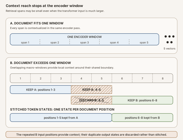
Scroll horizontally to inspect the diagram. The caption below provides a full text explanation.
This is not permission to improvise a duplicate rule. A version that averages overlap states, chooses centered states, or emits window-local chunk vectors is a different algorithm and should be documented and evaluated as such.
Reserve capacity for instruction and special tokens, prevent tokenizer truncation, and ensure every pooled span is fully covered. Overlap reduces one boundary problem; it does not create global context.
Long inputs also cost more to encode because transformer attention and intermediate activations grow with sequence length. Measure indexing throughput and peak memory with the actual model and window size.
Related techniques are not synonyms
| Technique | Context mechanism | Stored representation |
|---|---|---|
| Naive overlapping chunks | Repeats neighboring text in independently encoded chunks | One vector per overlapping chunk |
| Late chunking | Contextualizes a longer encoder input, then pools smaller spans | One vector per pooled span |
| Contextual text augmentation | Adds generated or extracted context to chunk text before embedding | Usually one vector per augmented chunk |
| ColBERT-style late interaction | Keeps multiple token vectors and scores them with query-time MaxSim | Multiple vectors per passage |
Late chunking and ColBERT’s “late interaction” share a word, not an operation. ColBERT retains token-level vectors and uses MaxSim, which finds each query token’s strongest similarity to a passage token before combining those matches. Late chunking instead pools contextual token states into a single vector per retrieval chunk. See the ColBERT paper for that separate design.
How to evaluate it on your corpus
Do not evaluate late chunking by hand-picking positive and negative words and asking whether absolute cosine scores moved in a preferred direction. Evaluate the retrieval system you intend to deploy.
Work through these four passes.
Pass 1: freeze the comparison
- Evaluation set: Freeze a document corpus, queries, and relevance judgments.
- Model path: Freeze model and tokenizer revisions, instructions, the chunker, boundaries, and query encoding.
Pass 2: state what the comparison isolates
- Target: Decide whether this is a context-only ablation or an end-to-end protocol comparison.
- Matched inputs: For a context-only test, hold fixed input IDs, special tokens, position inputs, pooled positions, pooling, and normalization. Vary only cross-span context or attention.
- Disclosure: If more than context changes, list every additional protocol difference.
Pass 3: measure rankings and costs
- Ranking quality: Compare nDCG@10, Recall@k, and MRR at the query level. Here, \(k\) means the chosen number of top results to inspect.
- Uncertainty: Resample defensible units such as queries or datasets while preserving known grouping and dependence.
- System cost: Report indexing time, peak memory, index size, and query latency.
Pass 4: inspect heterogeneity and generalization
- Subgroups: Stratify by document length, chunk size, cross-chunk dependency, and irrelevant surrounding context.
- Failures: Inspect queries that regress badly instead of relying only on the mean.
- Scope: State which corpora, models, and protocol choices the conclusion actually covers.
For a production decision, the relevant quantity is the control-relative retrieval change on representative data, not whether one illustrative cosine similarity increased.
Decision checklist
Late chunking may be worth testing
- Useful context often lives outside the target retrieval chunk.
- The embedding model exposes token states and a compatible pooling recipe.
- Several retrieval chunks fit inside one practical encoder window.
- Additional indexing cost is acceptable while query-time vector search stays unchanged.
Prefer the simpler baseline, or expect a smaller gain
- Chunks are already self-contained.
- Surrounding text is mostly irrelevant.
- Documents routinely exceed the usable window and local macro-context is insufficient.
- The provider exposes only an already-pooled embedding endpoint.
- Representative evaluation shows no robust ranking benefit for the added indexing cost.
Appendix A: reproduce and audit the result
The page bundle contains the current reproduction and verification script, the exact generator archived from the recorded model run, locked dependency graph, byte-identical test qrels, aggregate metrics, per-query metrics, top-ten rankings, run receipt, provenance manifest, and SciFact attribution. The archive lets the verifier confirm the generator hash recorded before this article-only revision. Model weights, corpus text, and caches remain uncommitted.
mrr_at_10 as the
field name for each individual query’s reciprocal rank. During review, those
per-query fields were renamed rr_at_10; no ranks, relevance labels, scores,
or metric values changed. The aggregate field remains mrr_at_10 because it is
the mean of the 300 per-query reciprocal ranks. The archived generator and the
run receipt preserve this history explicitly.
The committed receipts are much cheaper to inspect than re-running the model. From this bundle, the following standard-library-only cell prints the three aggregate rows and the late-minus-naive query counts:
import json
from pathlib import Path

results = json.loads(Path("receipts/aggregate.json").read_text())
for name in ("naive", "late", "whole_document"):
    row = results["methods"][name]
    print(
        name,
        f"nDCG@10={row['ndcg_at_10']['mean']:.4f}",
        f"Recall@10={row['recall_at_10']['mean']:.4f}",
        f"MRR@10={row['mrr_at_10']['mean']:.4f}",
    )

paired = results["paired_late_minus_naive_ndcg_at_10"]
print(
    "late minus naive:",
    paired["improved_queries"], "improved,",
    paired["tied_queries"], "tied,",
    paired["worse_queries"], "worsened",
)
Expected output:
naive nDCG@10=0.6414 Recall@10=0.7626 MRR@10=0.6123
late nDCG@10=0.6610 Recall@10=0.7776 MRR@10=0.6337
whole_document nDCG@10=0.6389 Recall@10=0.7592 MRR@10=0.6105
late minus naive: 49 improved, 229 tied, 22 worsened
Run the full model evaluation only when you need to recreate the embeddings and rankings. It downloads the checksum-pinned SciFact data and model files and took about eight minutes on the recorded Apple-silicon CPU run:
uv run --frozen reproduce.py --run --device cpu --batch-size 32 --threads 8
Before inference, the script validates the SciFact archive; model, tokenizer, and remote Python snapshots; the expected lockfile hash; and material installed package versions. The documented uv run --frozen command enforces the complete locked dependency graph. The receipt records the observed command, platform, versions, CPU settings, input hashes, protocol choices, phase timings, and output hashes. Deterministic-kernel mode is enabled, but the receipt does not promise bitwise identity across different hardware or math libraries.
Continuous integration (CI), meaning the automated checks run before publication, uses this offline command:
python3 reproduce.py --verify
That check binds the run to the script and lockfile, validates the frozen qrels hash, requires one complete ten-document ranking with unique document IDs for every query-arm pair, re-derives relevance labels and query metrics, re-runs the query bootstraps, and regenerates both empirical SVGs and their receipts byte for byte.
Appendix B: the formal definition
The five-step recipe in the main text is enough to implement the method. This appendix writes the same recipe compactly.
Let \(x\) be the actual in-window encoder sequence, including any chosen instruction and special tokens, and let \(a_i\) be its attention mask. Here \(x\) also stands for other fixed encoder inputs, such as position or token-type IDs where the model uses them. The transformer produces one contextual state for each encoded position:
\[ H = E(x,a) = \left[h_1(x,a), h_2(x,a), \ldots, h_m(x,a)\right]. \]Let \(S_j\) be the encoded positions assigned to retrieval chunk \(j\), with at least one position marked usable by the attention mask. For attention-mask mean pooling followed by L2 normalization, and assuming the pooled vector has nonzero finite length:
\[ \begin{aligned} \mu_j^{\mathrm{late}} &= \frac{\sum_{i \in S_j} a_i h_i(x,a)}{\sum_{i \in S_j} a_i}, \\ z_j^{\mathrm{late}} &= \frac{\mu_j^{\mathrm{late}}}{\lVert\mu_j^{\mathrm{late}}\rVert_2}. \end{aligned} \]The first line averages the usable contextual states in chunk \(j\). The second divides that average by its L2 length, producing the stored unit vector \(z_j^{\mathrm{late}}\).
For naive chunking, let \(x^{(j)}\), \(a^{(j)}\), and \(S_j^{(j)}\) describe chunk \(j\)’s separately encoded input, attention mask, and local pooled positions:
\[ \begin{aligned} \mu_j^{\mathrm{naive}} &= \frac{\sum_{r \in S_j^{(j)}} a_r^{(j)} h_r(x^{(j)},a^{(j)})}{\sum_{r \in S_j^{(j)}} a_r^{(j)}}, \\ z_j^{\mathrm{naive}} &= \frac{\mu_j^{\mathrm{naive}}}{\lVert\mu_j^{\mathrm{naive}}\rVert_2}. \end{aligned} \]The indices are different on purpose. A late position \(i\) is contextualized inside the longer input \(x\). A naive position \(r\) belongs to the separately encoded chunk input \(x^{(j)}\). These equations describe this reproduction’s pooling recipe. Another embedding model may specify different pooling or normalization.
Primary references
- Michael Günther et al., Late Chunking: Contextual Chunk Embeddings Using Long-Context Embedding Models, v3, 2024. Version 3 dated July 2025; accessed July 20, 2026.
- Jina AI, official Late Chunking implementation, pinned commit
1d3bb02. Commit-pinned source accessed July 20, 2026. - Michael Günther et al., Jina Embeddings 2: 8192-Token General-Purpose Text Embeddings for Long Documents, 2023.
- Jina AI,
jina-embeddings-v2-small-enmodel card, pinned revision44e7d1d. Revision-pinned source accessed July 20, 2026. - Nandan Thakur et al., BEIR: A Heterogeneous Benchmark for Zero-shot Evaluation of Information Retrieval Models, 2021.
- David Wadden et al., Fact or Fiction: Verifying Scientific Claims, 2020; see also the SciFact data license notice, accessed July 20, 2026.
- Omar Khattab and Matei Zaharia, ColBERT: Efficient and Effective Passage Search via Contextualized Late Interaction over BERT, 2020.