A Linear Nudge, a Nonlinear Wake
On this page 20 sections
Abstract. In this note, activation steering means additive residual-stream intervention: a controlled vector added to a model’s residual stream. That is one common steering primitive, not a definition of the whole field. A Jacobian lens is a corpus-average first-order map from that mid-network state toward later residuals and vocabulary dispositions. Before attributing a downstream effect to the meaning of a steering direction, requested-versus-realized fidelity under low precision, linear transport, and nonlinear model dynamics need to be separated.
(1) In Llama 3.3 70B Instruct, we applied three unselected Gaussian directions
after block 50 across eight prompts, varied dose from 0.5% to 30% of
residual RMS, and followed the signed response (the
half-difference of paired \(\pm\)dose runs) through the remaining 29 blocks. Protocol, plan, and decision rules were frozen
before outcomes
(a084caa).
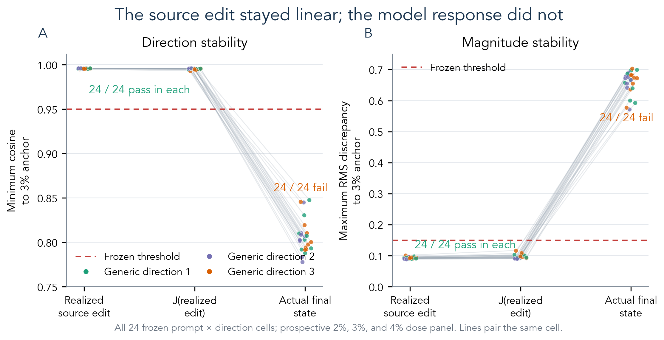
(2) On the frozen 2%/3%/4% panel, every one of the 24 prompt ×
direction cases kept a dose-linear source edit, while every final
hidden-state response failed both gates: direction drifted
(\(c_{\min}\) fell to 0.778–0.848, below 0.95) and dose-normalized size
mismatched (\(d_{\max}\) rose to 0.572–0.703, above 0.15). The fixed-J
projection of the realized edits stayed inside the same bounds as an algebraic
consistency reference, not as a claim that J predicted the model.
(3) Requested-versus-realized edit fidelity under
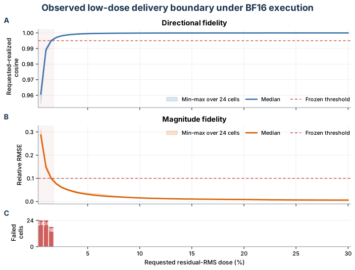
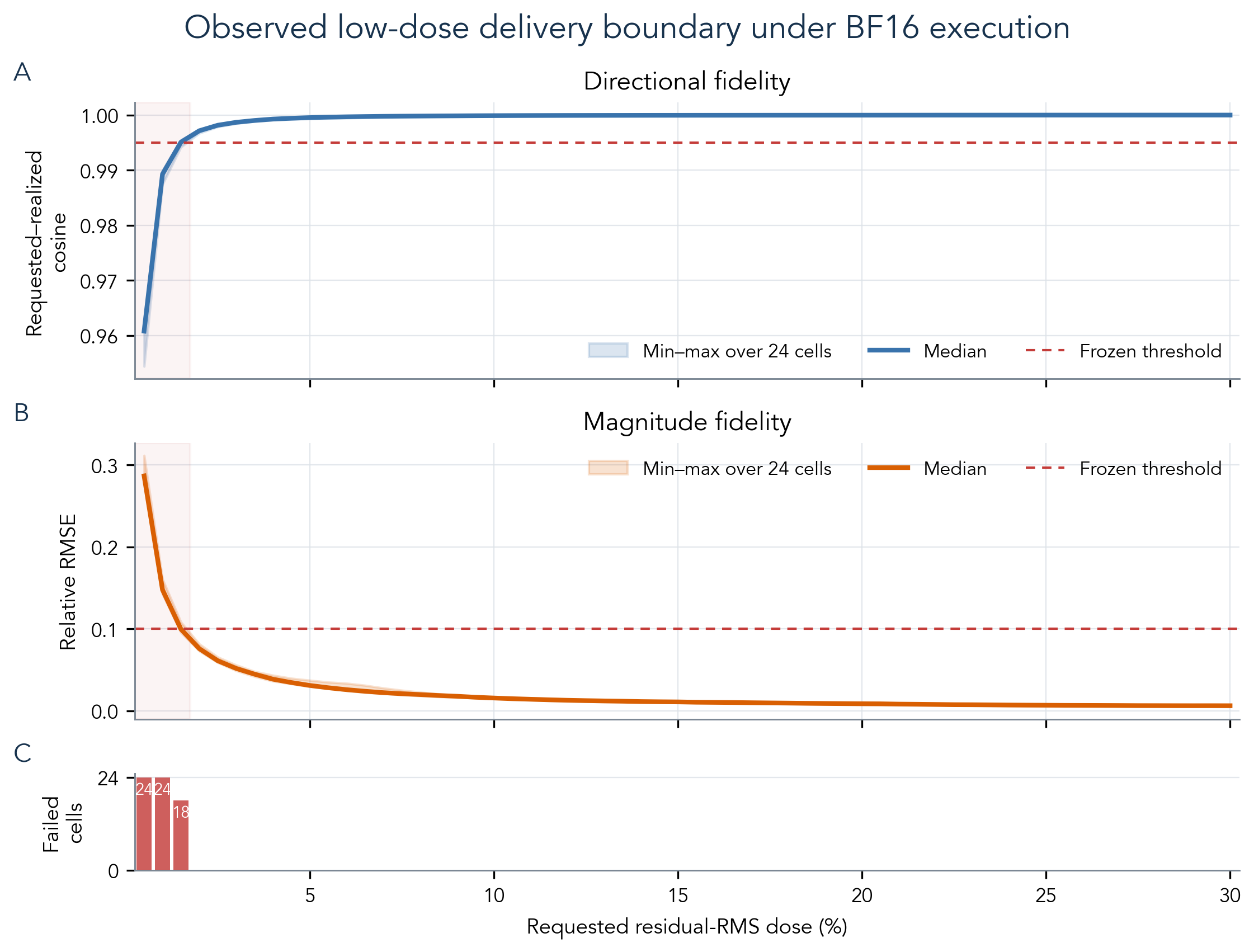
BF16 casting failed the frozen rule below 2% and
passed from 2% through 30% (the protocol’s short name for this check is
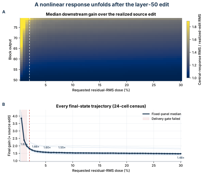
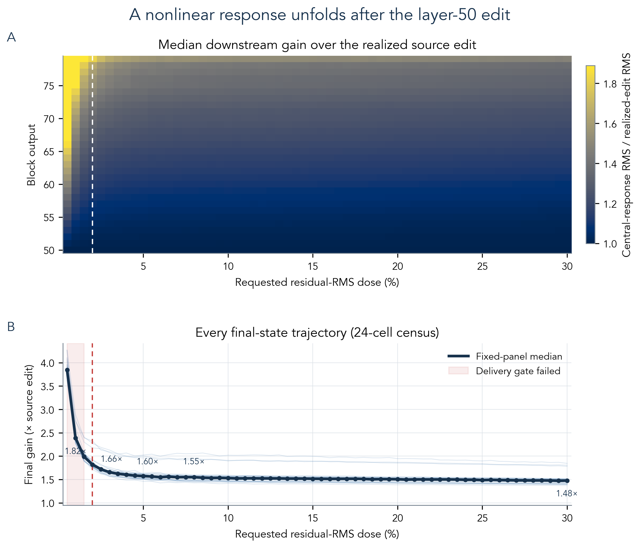
“delivery”). Median final-state RMS gain was 1.82x
at 2% and tapered to 1.48x at 30% over this fixed census.
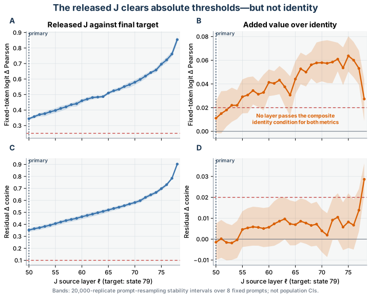
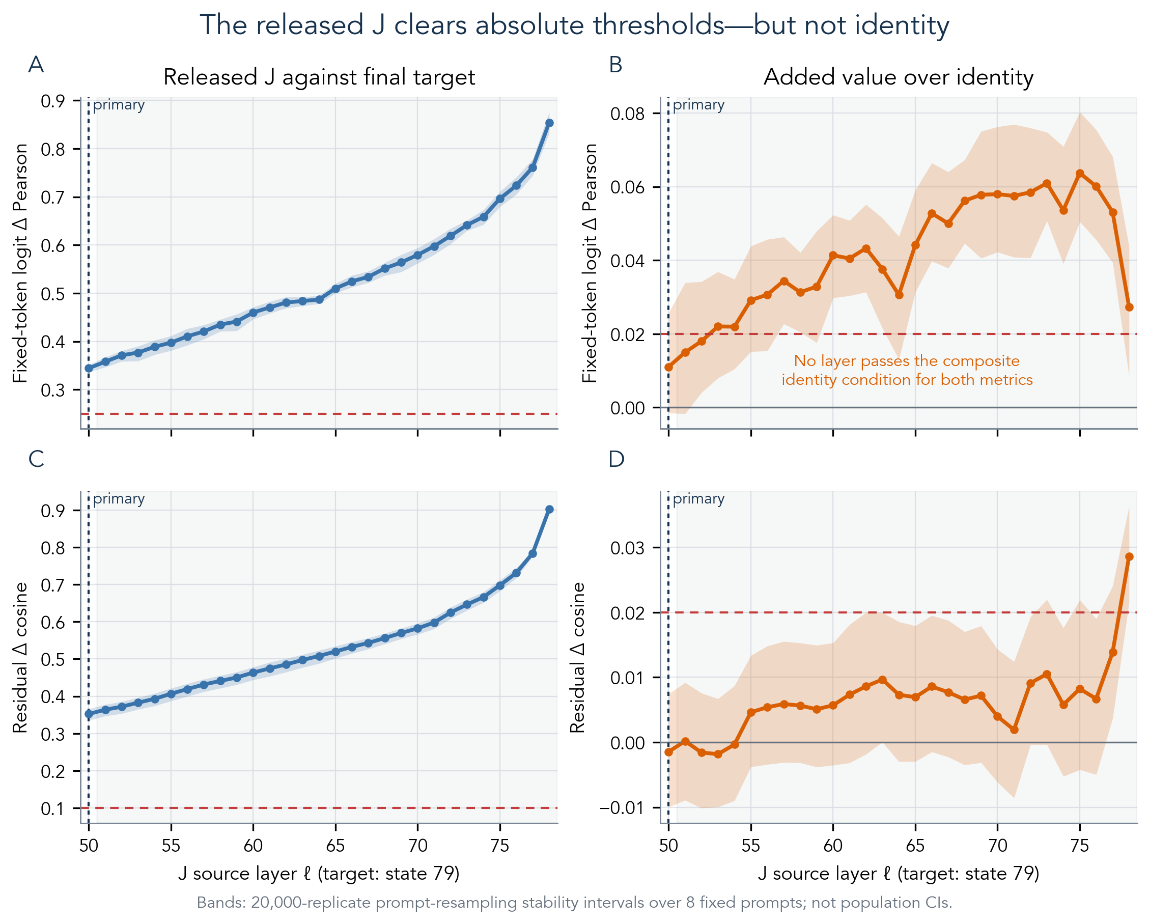
(4) At the primary layer-50 comparison, released J beat five
random-J maps but did not clear
added-value-over-identity (logit advantage 0.011, residual advantage slightly
negative).
Takeaway. Linear edit in, nonlinear hidden-state wake out, for these generic directions on this model. The result motivates an SAE-specific dose scan; it does not establish an SAE, behavioral, or consciousness claim.
Study status: complete (pre-outcome freeze
a084caa;
audited result release
fde24e9).
Experiment package:
experiments/consciousness_sae_signed_dose_scan.
Shipping table, sample records, and hashes are in the
appendix.
Reading routes: Main result → interpretation; measurement design → scoring rules; or artifact ledger → technical appendices. The Taylor discussion offers hypotheses for follow-up.
The Question
Activation steering changes a model from the inside. In the additive form studied here, the researcher adds a controlled vector to the hidden state carried between Transformer blocks instead of changing the prompt; contrastive activation addition is the canonical modern example (Rimsky et al., 2024). The field also includes adaptive, feature-targeted, and geometry-preserving variants, which this note does not test. The added vector can encode a proposed semantic direction, such as a sparse-autoencoder feature, or it can be deliberately generic, as in the experiment reported here.
A Jacobian is a local derivative: the high-dimensional analogue of a tangent line. A Jacobian lens (Gurnee et al., 2026) turns that idea into a reusable reference by averaging input-output Jacobians over many prompts and token positions. The result is one fixed linear map for each source layer: a corpus-average first-order approximation, not the exact Jacobian of the prompt under study. Gurnee et al. built the lens to surface verbalizable, vocabulary-oriented content; this note repurposes it as a transport benchmark for arbitrary residual perturbations, a different job from the one it was fit for. Whether averaged first-order maps carry useful structure is itself setting-dependent: relation-decoding work finds that mean Jacobian-based affine maps decode some relations well and others poorly (Hernandez et al., 2024).
This distinction matters because a downstream change can have several causes. The requested intervention may not land accurately in low-precision arithmetic. A well-delivered edit may propagate as the linear map predicts. Or the model’s remaining nonlinear blocks may reshape it. Before attributing a downstream effect to the meaning of a steering direction, these possibilities need to be separated.
Prior work, contribution, and non-claims
Prior work. Gurnee et al. introduce the Jacobian lens and connect mid-layer directions to later residual and vocabulary geometry (2026). Public fitting tooling and Llama maps come from Anthropic’s reference implementation (2026) and Neuronpedia’s Llama release (2026). Recent dose and steering work reports that intervention strength need not grow effects monotonically (Taimeskhanov, Vaiter, and Garreau, 2026) and that stronger SAE refusal steering can coincide with collateral over-refusal (O’Brien et al., 2025). An earlier Praxagent note asks whether SAE steering leaves a detectable J-space fingerprint under matched access models (Jones, 2026). This note does not invent the lens or the general fact that neural networks are nonlinear.
This note’s contribution.
- a prospectively frozen, target-masked signed dose scan on Llama 3.3 70B that retains requested edit, BF16-realized edit, fixed-J reference, and actual state separately at every dose and depth;
- a complete 24-cell census on the frozen
2%/3%/4%linearity panel, with identity and five random-J controls on the primary predictive comparison; - a public ledger in
tdj28/llm_selfref_prewith freeze and audited-release commits separated.
Not claimed.
- that SAE decoder directions, as a class, are nonlinear downstream;
- that any specific SAE feature has its published semantic interpretation;
- that generated behavior, deception, or consciousness-related vocabulary changed;
- that the corpus-average J outperforms simply carrying the residual change forward (it did not clear that frozen margin here).
Design in Brief
We tested this in
Llama 3.3 70B Instruct.
Immediately after transformer block 50, we applied three stress-test directions
to eight prompts, varied their magnitude from 0.5% to 30% of
residual RMS, and followed the response through the
remaining 29 blocks. The directions were unselected: independent Gaussian
vectors normalized to unit RMS, generated from
predeclared seeds and frozen before the experiment, with no step that picked
them for meaning, expected effect, or resemblance to any SAE feature. They test
the mechanics of perturbation transport rather than any concept.
What one measurement is
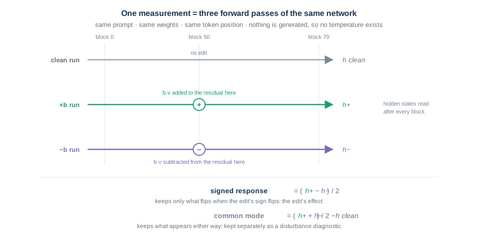
A “run” in this study is one deterministic forward pass, not a generation. The same network with the same weights reads the same fixed prompt; no tokens are sampled, so no temperature is involved anywhere. We record the hidden state the model computes at one fixed position (the continuation token, the final rendered prompt token) after each block.
For each prompt there is one clean run with no intervention. For each
direction and dose there are two edited runs, identical to the clean run in
every respect except one: immediately after block 50, the direction vector,
scaled to the requested dose, is added to (\(+b\) run) or subtracted from
(\(-b\) run) the residual state at that position before block 51 continues.
The model is therefore its own control. Any difference between runs at any
later block can only have come from that one injected vector, because nothing
else differs: weights, prompt, position, and arithmetic path are identical. The clean run
also sets the dose scale: a dose of 2% means the injected vector’s
RMS is 2% of the clean run’s layer-50 residual RMS
for that prompt. The frozen grid comes to 2,896 forward passes in total.
The paired edited runs act like pushing and then pulling the same knob. Any downstream change genuinely driven by the edit should flip sign between the two runs; anything that shows up either way (noise, or the model reacting to being disturbed at all) should not. Half the difference between the two runs keeps the flipping part and cancels the rest; we call that the signed response (the implementation’s name for it is the central contrast). The non-flipping part, measured as the midpoint of the two runs relative to an unedited run, is kept as a separate common-mode diagnostic. Because each \(+\)/\(-\) pair collapses into one curve, the census has 24 prompt × direction curves rather than 48 independent observations. Exact construction, provenance, dose grid, and pairing equations are in Appendix A.
 Source: this research note.
Credit: Timothy Jones / praxagent.
All rights reserved.
Source: this research note.
Credit: Timothy Jones / praxagent.
All rights reserved.
Diagram: how one measurement is built from three forward passes. This is a hand-drawn conceptual schematic, not a receipt-backed data figure; the exact pairing equations are in Appendix A.
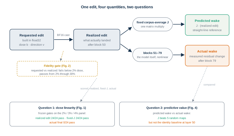
At every dose, the analysis retained four quantities: the edit requested in high precision; the edit realized after casting into BF16 activations (see requested-versus-realized fidelity); the downstream change from the fixed Jacobian map; and the downstream change the model actually produced. Separating requested from realized keeps low-precision rounding from being mistaken for nonlinear model dynamics.
 Source: this research note.
Credit: Timothy Jones / praxagent.
All rights reserved.
Source: this research note.
Credit: Timothy Jones / praxagent.
All rights reserved.
Diagram: the study decomposition (requested edit, realized edit, predicted wake, actual wake) and the two frozen questions asked of them. Conceptual schematic; the quoted pass counts are from the audited census reported in Figures 1–4.
Every decision rule (which doses count, which quantities are compared, and
the numeric thresholds for passing) was written down and committed to git
before any results were computed. The ordering matters: thresholds chosen
after seeing the data can make a “pass” or “fail” an artifact of where the
goalposts were placed, whereas rules frozen first let the experiment genuinely
come out either way. Concretely, the frozen rule says: once a small edit
demonstrably landed intact, the model’s final response counts as linear only
if scaling the dose across 2%/3%/4% scales the response by the same
factor while keeping nearly the same direction, within the two numeric bounds
defined below. Failing that rule means the local-linear description broke by a
prespecified margin on this panel. It does not mean “networks are nonlinear”
in general, and it is not an estimate of how often this happens across other
models or directions.
The Linear Edit and the Nonlinear Wake
What “linear” means in this note
Imagine a dimmer switch. If the response is dose-linear, turning the dose
from 2% to 4% should roughly double the size of the change while leaving
its direction alone. In vector language: the hidden-state response at dose
\(b\) should look like \(b\cdot v\) for one fixed direction \(v\).
Nonlinear, here, means that rule fails in a measured way: as dose changes, the response rotates (direction drifts) or its size stops tracking the dose (amplification or compression). We are not using “nonlinear” as a vibe word for “the network has nonlinear layers.” Transformers are nonlinear by construction. The question is whether this dose–response curve stayed close enough to a straight line through the origin on a small, prechosen panel.
A cell is one prompt paired with one generic direction: 8 prompts × 3 directions = 24 cells. For each cell we track the signed response across dose (the \(+\)dose run minus the \(-\)dose run, halved, as defined in the design section), so the 24 cells are 24 curves, not 48 independent signed runs.
We apply the same linearity test to three quantities in each cell:
- Source: the edit that actually landed after block 50.
- Fixed J: that same realized edit pushed through the corpus-average Jacobian map (an algebraic straight-line reference).
- Actual final: the model’s real residual change after block 79.
How we scored pass versus fail
The frozen panel is \(B=\{0.02,0.03,0.04\}\) (2%, 3%, 4%), with 3% as
the anchor. That panel is the first three-dose window where every source edit
already cleared the requested-versus-realized fidelity checks; Figure 2 shows
that boundary.
Every response vector \(x_b\) below is built from the paired runs described in the design section: for the source, it is the signed response measured right after block 50 (the half-difference of the \(+b\) and \(-b\) runs at the continuation position); for the actual final, the same half-difference measured after block 79; for fixed J, the source vector pushed through the released linear map. No new runs, prompts, or sampling are involved; the three quantities are three readouts of the same 2,896 deterministic forward passes.
For a response vector \(x_b\) at dose \(b\), form the dose-normalized vector
\[ q_b = \frac{x_b}{s_b}. \]The divisor \(s_b\) is the size of the input being scaled. For the source
edit, \(s_b\) is the requested dose fraction (0.02, 0.03, 0.04). For J
and the actual final state, \(s_b\) is instead the measured
RMS size of the edit that actually landed at block
50, expressed as the same kind of fraction. The reason for the switch: those
two quantities are downstream of the realized edit, so the fair question is
“per unit of edit that landed, what came out?”, not “per unit of edit we
asked for.” Dividing by \(s_b\) puts every dose on that per-unit scale. If
doubling the landed edit exactly doubled the downstream response without
turning it, the normalized vectors \(q_b\) at 2%, 3%, and 4% would all
be the same vector; how far they spread apart is what the two statistics below
measure.
Two statistics then ask whether the \(q_b\) stay near the 3% anchor
\(q_{0.03}\):
- \(c_{\min}\) is directional agreement (1 means identical direction).
- \(d_{\max}\) is relative size mismatch after dose normalization (0 means identical scale and shape). The implementation calls \(d_{\max}\) “slope discrepancy.”
A cell passes for a quantity when both frozen gates hold:
\[ c_{\min}\ge 0.95 \quad\text{and}\quad d_{\max}\le 0.15. \]Fail either gate and that quantity is scored nonlinear on this panel. Exact construction of \(x_b\) (signed branches, common-mode diagnostic) is in Appendix A.
0.95
tolerates directional wobble inside roughly an 18° cone, and a discrepancy
ceiling of 0.15 sits comfortably above the roughly 0.10 relative deviation
that BF16 delivery alone induces in the source edits, so a faithfully landed
edit cannot fail the panel merely because of rounding noise. What protects the
conclusion is not the exact numbers but two facts: the thresholds were
committed before any outcome was seen, and the results landed nowhere near
them. Sources and fixed-J scored \(c_{\min}\ge 0.993\) and
\(d_{\max}\le 0.117\); actual finals scored \(c_{\min}\le 0.848\) and
\(d_{\max}\ge 0.572\). Any cosine floor between 0.85 and 0.99, and any
discrepancy ceiling between 0.12 and 0.57, produces the identical
24/24-versus-0/24 split.
 Source: this research note.
Credit: Timothy Jones / praxagent.
All rights reserved.
Source: this research note.
Credit: Timothy Jones / praxagent.
All rights reserved.
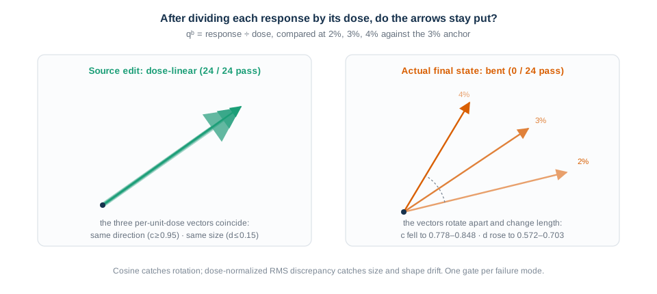
Diagram: the two failure modes the frozen gates test, drawn as dose-normalized vectors \(q_b\). Conceptual schematic: arrow geometry is illustrative; the quoted numeric ranges are the audited census values also shown in Figure 1.
import numpy as np

B = (0.02, 0.03, 0.04)
ANCHOR = 0.03

def rms(x: np.ndarray) -> float:
    return float(np.sqrt(np.mean(np.square(x))))

def cosine(a: np.ndarray, b: np.ndarray) -> float:
    return float(np.dot(a, b) / (np.linalg.norm(a) * np.linalg.norm(b)))

def dose_linearity_gates(
    x_by_dose: dict[float, np.ndarray],
    s_by_dose: dict[float, float],
    *,
    cosine_min: float = 0.95,
    slope_max: float = 0.15,
) -> tuple[float, float, str]:
    """Return (c_min, d_max, 'pass'|'fail') for one cell and one quantity."""
    q = {b: x_by_dose[b] / s_by_dose[b] for b in B}
    q_anchor = q[ANCHOR]
    c_min = min(cosine(q[b], q_anchor) for b in B)
    d_max = max(rms(q[b] - q_anchor) / rms(q_anchor) for b in B)
    status = "pass" if c_min >= cosine_min and d_max <= slope_max else "fail"
    return c_min, d_max, status

# Example call for one prompt × direction cell:
# c_min, d_max, status = dose_linearity_gates(source_x, source_s)
What the census found
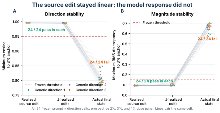
Against that frozen first-order benchmark, the split was complete: 24 of 24 source edits passed both gates, 24 of 24 fixed-J references also passed, and 0 of 24 actual final-state responses did.
| Quantity | \(c_{\min}\) (need \(\ge 0.95\)) | \(d_{\max}\) (need \(\le 0.15\)) | Cells passing |
|---|---|---|---|
| Realized source edit | 0.995–0.996 |
0.089–0.101 |
24 / 24 |
| Fixed J of that edit | 0.993–0.996 |
0.090–0.117 |
24 / 24 |
| Actual final state | 0.778–0.848 |
0.572–0.703 |
0 / 24 |
So the finals did not fail by a hair on one metric. In every cell they failed
both rules: the dose-normalized response rotated away from the 3% anchor
(cosine well below 0.95) and its per-unit-dose size/shape drifted far past
the 0.15 ceiling. Source and fixed-J curves, by contrast, sat near cosine
1 with only about 0.1 relative discrepancy.
In plain English: at the intervention site the delivered edit behaved like a
dimmer. After 29 more blocks, turning the dose from 2% to 4% no longer
gave “same arrow, twice as long.” The arrow bent, and the length stopped
tracking dose. The fixed Jacobian cannot invent that failure by itself: a
fixed linear map would preserve exact proportionality, and here the
approximately proportional source curves also stayed inside both numerical
bounds after projection. The curvature therefore sits in the model’s mapping
from the realized post-block-50 edit to the post-block-79 residual, not in
dose-dependent mangling of the source edit. Fixed J is an algebraic and
implementation control here; it is not evidence that J predicted the model
accurately. Predictive accuracy is tested separately in Figure 4.
Table: frozen-panel linearity census ranges across the 24 cells. Provenance: fig-1-linearity-census.receipt.json · provenance.json.
Figure 1 shows the complete census rather than an average. Its three horizontal
categories are the realized source edit, J applied to that realized edit, and
the actual final state. The left panel plots \(c_{\min}\) against the 0.95
floor; the right plots \(d_{\max}\) against the 0.15 ceiling. Each connecting
line is one prespecified prompt × direction cell.
 Source: this research note.
Credit: Timothy Jones / praxagent.
All rights reserved.
Source: this research note.
Credit: Timothy Jones / praxagent.
All rights reserved.
Figure 1: source linearity versus actual downstream curvature. Each line is one of 24 prompt × direction central-contrast curves over the prespecified 2%/3%/4% panel. In these data, the fixed linear operator left the near-proportional delivered curves within both numerical bounds; that panel is a consistency reference, not a test of predictive accuracy. The model's actual final hidden states satisfy neither criterion in any cell. Dashed lines mark thresholds fixed before outcomes. Provenance: receipt · plot_signed_dose_scan_results.py · provenance.json. Verify (needs the on-request audited summary): python3 plot_signed_dose_scan_results.py --summary CALIBRATION_SUMMARY.json --output-dir . --verify --post index.md.
Requested-versus-realized edit fidelity under BF16
“Delivery” is not a standard ML term. It is this study’s short name for a simple fidelity check: does the intervention vector we requested match the vector that was realized in the residual after casting into the model’s number format?
That format here is BF16 (bfloat16): a 16-bit floating-point type with FP32-like range but much coarser precision, so many float32 values round to the same BF16 number. For bit layouts, casting demos, and accumulation swamping, see the Deep Dive BF16, FP16, and FP32: Precision, Range, Swamping, and Determinism. The protocol builds the requested edit in float32 along a unit-RMS direction, then casts it into the BF16 residual hook. Write \(e^{\mathrm{req}}\) for the intended vector and \(e^{\mathrm{real}}\) for the change actually present after the hook. If rounding were negligible, those two would nearly match.
We score that match with the same two geometric ideas as linearity, now comparing request to realization at a single dose:
\[ \cos\!\big(e^{\mathrm{req}},e^{\mathrm{real}}\big) \ge 0.995, \qquad \frac{\operatorname{RMS}\big(e^{\mathrm{real}}-e^{\mathrm{req}}\big)} {\operatorname{RMS}\big(e^{\mathrm{req}}\big)} \le 0.10. \]The full gate also checks both signed branches, their signed response (the half-difference defined in the design section), and the common-mode response. Fail any piece and that cell fails the fidelity check at that dose.
# Uses the same rms() / cosine helpers as the linearity sketch above.
def requested_realized_ok(
    e_req, e_real, *, cos_min=0.995, rel_rmse_max=0.10
) -> bool:
    return (
        cosine(e_req, e_real) >= cos_min
        and rms(e_real - e_req) / rms(e_req) <= rel_rmse_max
    )
Why this matters: if a tiny requested dose mostly rounds away, a “nonlinear” downstream curve could just be noise from a mangled source edit. The fidelity check asks whether the source edit is faithful enough to blame the model for what happens next.
What we observed
At very small magnitudes, that rounding is not negligible. In this exact model,
hook, prompt panel, and set of generic directions, the three smallest dose
levels did not meet the predefined fidelity bounds. All 24 cells failed the
full paired-branch rule at 0.5% and 1%, and 18 of 24 did so at 1.5%.
Every cell passed from 2% through 30%.
At 2%, requested-versus-realized cosine had a median of 0.997, while median
relative RMSE was 0.076. Passing does not mean requested and realized edits
were bit-identical. It does show that the final-state nonlinearity on the
2%/3%/4% panel cannot be blamed on the low-dose fidelity failure seen
below 2%. The boundary is consistent with BF16 rounding, but the experiment does not
isolate rounding from other implementation details such as the casting path,
kernel ordering, or fused operations. It is an empirical property of this
implementation and panel, not a universal BF16 limit; a datatype and hook-path
ablation (FP32, FP16, alternative hook implementations) would be the direct
mechanism test.
 Source: this research note.
Credit: Timothy Jones / praxagent.
All rights reserved.
Source: this research note.
Credit: Timothy Jones / praxagent.
All rights reserved.
Figure 2: low-dose requested-versus-realized fidelity under this BF16 setup (file stem fig-3-bf16-delivery-floor; “delivery” is the protocol nickname). The upper curves show the central signed estimate; the bottom strip applies the complete rule to both signed branches, their central contrast, and their common-mode response. Pale envelopes are the observed minimum and maximum across the fixed census (all 24 prespecified prompt × direction cells), not confidence intervals. Provenance: receipt · plot_signed_dose_scan_results.py · provenance.json.
Watch the Wake Develop Across Depth
At each state, gain is the root-mean-square magnitude of the signed
response, \((h_{+}-h_{-})/2\), divided by the RMS magnitude of the realized
signed source edit. It is 1x at state 50 by construction. A gain of 1.8x,
for example, means the downstream signed response is 80% larger in RMS than
the edit that landed. Median gain generally accumulated through later blocks,
although individual trajectories were not uniformly monotone. Every tested
trajectory ended above 1x.
The median final-state gain was 1.82x at 2%, 1.66x at 3%, 1.60x at
4%, 1.55x at 8%, and 1.48x at 30%. Relative amplification was
generally larger at lower eligible doses (doses where every cell passed the
requested-versus-realized checks), though the complete half-point dose series
was not perfectly monotone.
Figure 3 makes the depth and dose axes explicit. The upper heatmap runs dose horizontally and post-block state vertically; the lower panel shows final-state gain across dose for every one of the 24 cells, with their median emphasized.
 Source: this research note.
Credit: Timothy Jones / praxagent.
All rights reserved.
Source: this research note.
Credit: Timothy Jones / praxagent.
All rights reserved.
Figure 3: the measured hidden-state response from the intervention point to the final block (file stem fig-2-dose-depth-arc). The heatmap uses fixed-panel medians (the median across the same prespecified 24 cells at each dose and layer); the lower panel retains every trajectory. These are descriptive census summaries of exactly these 24 cells, not population estimates. Provenance: receipt · plot_signed_dose_scan_results.py · provenance.json.
Did the Jacobian Lens Predict the Wake?
Cross-dose curvature and predictive usefulness at one dose are logically independent: a response can bend as dose changes while a first-order map still captures useful structure at a fixed dose. Figure 1 used J only as a linear algebra reference. Predictive accuracy requires a different test: compare J’s prediction with the final response and ask whether it beats cheap alternatives. We used two: identity, which carries the observed source-state change forward unchanged (a geometry-free transport baseline, not a vocabulary readout such as a logit lens or tuned lens (Belrose et al., 2023)), and five prespecified random-J controls, which apply seeded sign and coordinate permutations to the released map.
The layer-50 source state was selected in advance for the primary comparison.
On this fixed 3% panel, the released J cleared the absolute thresholds and
decisively beat the strongest of five random maps in both metrics. For
fixed-token logit correlation (agreement between predicted and observed score
changes for 2,048 prespecified vocabulary tokens), real J scored 0.344; its
advantage over the strongest random map was 0.286, with a 95% fixed-panel
stability lower bound of 0.271. In residual space, the corresponding advantage
was 0.337, with a lower bound of 0.321.
Identity was the harder baseline. J’s logit advantage over identity was only
0.011, with a lower bound of -0.0015, below the predefined 0.02 margin.
Its residual-space advantage was slightly negative (-0.0015). No tested
source-state layer cleared the added-value-over-identity margin in both spaces.
The bounded conclusion is therefore precise: the released map contains
structure beyond these five randomizations, but it did not show added value
over simply carrying the residual change forward unchanged.
This comparison cannot separate two explanations for that null: that first-order transport itself adds little for these directions, or that corpus averaging washes out prompt-local structure that a per-prompt Jacobian would capture. A prompt-specific Jacobian baseline, run on the same cells, is the natural next control and was not part of this study.
For Figure 4, each horizontal position has a different source-state layer but the same target. At source layer \(\ell\), both \(J_\ell\) and identity receive the observed signed residual change after block \(\ell\) and predict the post-block-79 change. Only layer 50 is the intervention site. Layers 51–78 are shorter-horizon diagnostics after the model has already transformed the edit.
 Source: this research note.
Credit: Timothy Jones / praxagent.
All rights reserved.
Source: this research note.
Credit: Timothy Jones / praxagent.
All rights reserved.
Figure 4: prediction from successive source states to one fixed target. For each source layer \(\ell=50,\ldots,78\), \(J_\ell\) and identity receive the observed central residual change after block \(\ell\) and are compared with the same post-block-79 target. Layer 50 was selected in advance for the primary comparison; layers 51–78 are descriptive shorter-horizon diagnostics, not additional intervention sites. Bands are fixed-panel stability intervals obtained by resampling the eight prompts and do not support population-level inference. Provenance: receipt · plot_signed_dose_scan_results.py · provenance.json.
Implications for SAE Intervention Studies
The measurement design transfers to an SAE-specific study; the dose boundary
does not. A direct extension would replace the generic vectors with target SAE,
matched-SAE, and norm-matched generic directions, then rerun the
requested-versus-realized fidelity and common-mode checks for every vector.
The 2%/3%/4% panel is only a
candidate calibration starting point. Any semantic or behavioral extension
would also need its own controls and never-intervened counterfactual branch.
The generic-direction anomaly motivates that experiment; it does not confirm
an SAE mechanism. The target features, prompts, dose panel, semantic endpoints,
and analysis rules would need to be specified before their outcomes are
inspected.
Two cheaper follow-ups would sharpen the present result before any semantic extension: the datatype and hook-path ablation named above, which would turn “consistent with BF16” into a mechanism test, and a small public notebook that exports the requested edit, realized edit, fixed-J projection, and actual final residual for one prompt, one direction, and one layer at each dose, so the study’s central decomposition can be audited in minutes rather than hours.
Interpretation
Five conclusions follow from the experiment:
- this setup has an observed low-dose requested-versus-realized fidelity
boundary under BF16 casting, with universal passage beginning at
2%for the tested generic directions; - above that boundary, the realized edit remains dose-linear over the primary
2%/3%/4%panel, and the approximately proportional curves empirically remain within both bounds after fixed-J projection; - the actual final residual state changes direction and scale enough to fall outside both predefined linearity bounds in every cell;
- the full arc shows a dose-dependent transformation generally accumulating through the remaining blocks; and
- the released J beats five randomized maps but does not clear the stronger added-value-over-identity rule at any tested source-state layer.
These conclusions apply to the 24 tested prompt × direction combinations and to hidden-state dynamics. The experiment did not test generated behavior, SAE features, deception, or consciousness-related vocabulary.
The depth arc localizes where the first-order description stops being adequate; it does not identify the mechanism that bends the trajectory. Mechanistic explanations suggested by this pattern are hypotheses for a new study whose mechanism test is specified before data inspection.
Taken together, the result is both sharp and bounded: linear edit in, nonlinear hidden-state wake out. The corpus-average Jacobian sees nonrandom structure in that wake, but it does not outperform the simplest strong baseline: carrying the residual change forward unchanged.
Discussion: A Taylor-Series View of the Result
This section steps back from the audited numbers and asks what kind of object a Jacobian lens is, and why the observed split (every source edit linear, every fixed-J projection linear, every actual final state bent) is exactly the pattern a linearization story predicts. Everything here is interpretation; the census results above stand on their own, and the hypotheses below would need their own prespecified tests.
The fixed-J pass is a consistency reference. Exact proportionality is preserved by every fixed linear map: if \(x_b=bv\), then \(Jx_b=bJv\). For approximately proportional inputs, however, a matrix can amplify the deviations; passage through a finite cosine/RMS gate is not guaranteed. Here the realized edits and their released-J projections both passed empirically. The actual final states failed, locating a dose-dependent change in the executed downstream computation.
A local Jacobian supplies the first-order term. Write \(F\) for the function taking the post-block-50 residual to the post-block-79 residual. For an edit \(e\) around the clean state \(h\),
\[ F(h+e) = F(h) + J(h)\,e + \tfrac{1}{2}\,e^{\top}H(h)\,e + \cdots, \]where \(J(h)\) is the local Jacobian and \(H(h)\) the second-derivative term.
The experiment records the signed branches and centers their contrast as
\((F(h+e)-F(h-e))/2\). A prompt-local Jacobian would predict a response
proportional to dose. The released lens instead averages Jacobians across
other prompts and positions. The signed responses fail the dose-linearity
gates at 2%–4% RMS; that establishes a departure from proportionality
in this implementation, without isolating smooth higher-order dynamics
from finite-precision effects.
Two sources of approximation remain unresolved. First, truncation: it omits every term past the first. Second, expansion point: it is not even \(J(h)\) for the prompt under study but a Jacobian averaged over other prompts and positions. The Figure 4 null (J failing to beat identity) could come from either. The prompt-specific Jacobian baseline named above is the control that separates them, and there is a reasonable chance that fixing the expansion point buys more than adding a derivative order.
Identity is not a dumb baseline; it is the free part of the first-order term. Because of the residual stream, the true Jacobian has the form \(I + \text{(block contributions)}\): skip connections carry the edit forward unchanged at no cost. Identity is that free part alone. The finding that the corpus-average J could not beat it says the learned, averaged remainder of the first-order term added nothing detectable for these generic directions.
Would a second-order lens be superior? In principle yes; as a shipped
artifact, no. The first-order lens is an 8192 × 8192 matrix: about 67
million numbers. The second-order term is an 8192 × 8192 × 8192 tensor:
roughly \(5.5\times 10^{11}\) numbers, on the order of a terabyte per source
layer in BF16. What is feasible: Hessian-vector products computed on
demand by double backpropagation, which give \(e^{\top}H\,e\) for a specific
edit without materializing \(H\), and low-order polynomial fits along a fixed
direction, since the whole dose curve is then a function of one scalar.
Falling gain does not identify the correction. Median final-state gain
fell from 1.82x at 2% to 1.48x at 30%. This is compatible with
saturation and with a negative higher-order correction. For example,
\(F(e)=ae-be^3\), with \(a,b>0\), has signed response per unit dose
\(a-be^2\), which decreases over the range where it remains positive.
The gain curve alone therefore does not choose between a polynomial
correction and a saturating response. Fitting directional models on one
dose panel and checking them on held-out doses would test that distinction.
Why would smaller doses be amplified more? At first glance the gain
ordering looks backwards. It is not: the absolute wake still grows with
dose (a 30% edit moves the final state far more than a 2% edit); what
falls is the amplification per unit of delivered edit. The roughly 1.8x value is the gain at the smallest dose that passed
the requested-versus-realized fidelity rule. It is not an established
local-Jacobian gain: the 2%–4% panel failed dose-linearity, and the
smaller doses failed the fidelity rule. Several mechanisms could contribute
to the lower gain at larger doses. First, normalization compression:
Llama applies RMSNorm on the way into every block, dividing the residual by
its own overall scale. A tiny edit leaves that scale essentially untouched
and rides through; a 30% edit measurably inflates the very norm it is
divided by, so the network re-scales it downward everywhere downstream.
Second, attention saturation: small perturbations move pre-softmax scores
within their locally linear range, while large ones push attention patterns
toward saturated, nearly winner-take-all configurations whose marginal
sensitivity is lower. Third, trained robustness: a model trained on
enormous data has seen its own representational noise and may have learned
broadly contractive dynamics around its typical activations, so the farther
an edit pushes the state off that manifold, the harder the remaining blocks
pull back per unit of push. All three are hypotheses, not measurements. The
first is also the most testable: recompute gain after accounting for the
measured layer-wise norm inflation, or deliver the edit as a norm-preserving
rotation instead of an addition and check whether the dose profile of gain
flattens. The fidelity gate also bounds the discrepancy between requested and
realized edit sizes from 2% through 30%. It does not by itself
prove that the choice of denominator has zero effect on the gain curve;
recomputing both normalizations would quantify that sensitivity.
These framings are hypotheses. The census established where the first-order description stops being adequate for these directions on this model; the mechanism that bends the trajectory, and whether any of the candidate “superior lenses” would capture it, is a question for a study whose test is frozen before its outcomes are inspected.
Reproducibility And Artifact Ledger
Compact map for readers who already know what they want. Sample records and the teaching inventory are in the appendix.
| Artifact | Link |
|---|---|
| Experiment package | experiments/consciousness_sae_signed_dose_scan |
| Pre-outcome freeze | a084caa |
| Audited result release | fde24e9 |
| Frozen plan directory | dose_scan_v1_plan_20260716 |
| Compact replication record | …/signed-dose-a084caa-wl8obvtuq0ax8t-v2-audit-recovery-c9 |
| Protocol | docs/…/PROTOCOL.md |
| Result summary | RESULT_SUMMARY.md |
| Figure generator (sanitized post bundle) | plot_signed_dose_scan_results.py (SHA-256 0e9db35a…; publication copy of the generator committed upstream with the figure package at f5e906e, with machine-local receipt paths replaced by basenames) |
| Post-wide number manifest | provenance.json |
| Llama 3.3 70B Instruct | revision 6f6073b… (gated) |
| Neuronpedia J-lens config | revision a4114d7… |
Table: compact ledger. Freeze and release commits are separated on purpose. The 2.23 GB raw residual tree stays off-repository; its inventory SHA-256 is in the appendix.
Technical Appendices
Appendix: release inventory
a084caa)
before outcomes. The audited public package is
fde24e9
in tdj28/llm_selfref_pre. C9
recomputed the audit from the unchanged raw tree with zero fresh model
forwards.
| What we shipped | In plain English | For specialists | License / access |
|---|---|---|---|
| Experiment code and gates | Scripts that build, validate, run, and audit the scan | experiments/consciousness_sae_signed_dose_scan |
open (repo license) |
| Frozen plan | The pre-outcome protocol bytes | dose_scan_v1_plan_20260716; plan manifest field plan_manifest_sha256 79810742…63c51d |
open |
| Compact audit package | What a reader needs without the raw tensors | …/audit-recovery-c9; audit status pass |
open |
| Audited summary (26.8 MB) | Machine-readable census behind the figures | SHA-256 b490b101c112f774ae7bffc9c54294a70b91c874c4cee78eddaa7890446c08f6 |
on-request (too large for git; bound by PUBLICATION_COMPLETE.json) |
| Raw residual tree (2.23 GB) | Full archived arcs for independent replay | inventory SHA-256 9fc8c8ffe5f8d34f8ddba863c11fff7370ef3644c1fad0139f96e39a4c8fbfc0 |
withheld / on-request (volume retention; not in git) |
| Empirical figures | The four plots in this note | per-figure .receipt.json in this post bundle; index figure-receipts-index.json |
open (bundled here) |
| Llama 3.3 70B Instruct | Base weights for the run | revision 6f6073b423013f6a7d4d9f39144961bfbfbc386b |
gated (Llama Community License) |
| Neuronpedia J-lens maps | Corpus-average \(J_\ell\) used as reference | revision a4114d7752d11eb546e6cf372213d7e75526d3a1 |
publicly released (see HF card) |
Table: what "complete" means for this release. Middle column is plain language; right columns carry specialist pins and access conditions.
Open a record: compact publication marker
Plain English. The public package seals that the audit finished from the unchanged raw tree and records the hashes a skeptic should match.
Technical. PUBLICATION_COMPLETE.json in the compact replication record:
status = complete_atomic_audit_only_recovery;
summary_file_sha256 = b490b101…08f6;
audit_receipt_sha256 = 176e2f7e…ee1;
run id signed-dose-a084caa-wl8obvtuq0ax8t-v2.
Open a record: linearity census receipt
Plain English. Figure 1’s numbers are not typed by hand. A receipt lists every plotted range and failure count.
Technical. fig-1-linearity-census.receipt.json:
actual_final_failure_count = 24;
realized_source_failure_count = 0;
j_of_realized_failure_count = 0;
source summary SHA-256 b490b101…08f6.
Appendix A: Exact Test
The experiment used Meta’s Llama 3.3 70B Instruct
checkpoint
at revision 6f6073b… and Neuronpedia’s Llama-specific Jacobian-lens
release
at revision a4114d7…. Neuronpedia generated the maps with Anthropic’s
reference method,
averaging derivatives over 125 completed WikiText prompts of at most 128
tokens. They were not estimated from this study’s prompts or outcomes.
The three stress-test directions were independent standard-normal vectors in
the 8,192-dimensional residual space, normalized to unit
RMS and fixed by predeclared seeds. There was no
semantic or SAE-based selection, rejection for outcome behavior, or post-hoc
sign flip. Dose ran from 0.5% to 30% of residual RMS
in 0.5-percentage-point increments. The prompts, directions,
primary dose panel, and decision rules were fixed before outcomes were opened.
For prompt \(p\), direction \(v\), and magnitude \(b\), the two signed branches produce the realized signed source edit (the quantity the implementation calls the central contrast)
\[ e_b = \frac{h^{\mathrm{post50}}_{+b}-h^{\mathrm{post50}}_{-b}}{2}. \]The midpoint relative to the clean branch was retained as a separate common-mode diagnostic. The two signed branches therefore form one paired measurement. A linearity cell is one prompt × direction curve across dose, giving 24 cells rather than 48.
For a realized layer-50 edit \(e_b\), the fixed lens supplies
\[ \Delta h_{79}^{J} = J_{50}\,e_b. \]The released \(J_\ell\) is an 8192 × 8192 corpus- and position-averaged
input-output Jacobian from the post-block-\(\ell\) residual to the post-block-79
residual. It has no prompt-specific conditioning, intercept, or centering term.
The row-vector implementation is \(e_bJ_{50}^{\mathsf T}\). Because the same
linear operator is used at every dose, exact source proportionality would be
preserved automatically. The realized curves were only approximately
proportional, so remaining within the numerical bounds after J projection is an
empirical consistency check. Figure 4 separately evaluates prediction against
the observed target state and against identity and random-map controls.
The prespecified primary panel (the doses and decision rules committed before the
results were examined) compared the dose set
\(B=\{0.02,0.03,0.04\}\), with 3% as the anchor. For a response vector
\(x_b\), define the dose-normalized vector \(q_b=x_b/s_b\). For the realized
source, \(s_b\) is the requested BF16 edit’s residual-RMS fraction; for J and
the actual final response, \(s_b\) is the realized source edit’s residual-RMS
fraction. The two implemented statistics were
Each prompt-direction cell required \(c_{\min}\ge 0.95\) (the dose-normalized
vector kept nearly the same direction as the 3% anchor) and
\(d_{\max}\le 0.15\) (its component-wise RMS deviation from the anchor stayed
small). These are vector-valued dose-response checks; “slope discrepancy” is
the implementation’s name for \(d_{\max}\).
Realized-source and J-projected curves had minimum cosine between 0.993 and
0.996 and maximum slope discrepancy between 0.089 and 0.117. Actual-final
curves had minimum cosine between 0.778 and 0.848 and maximum slope
discrepancy between 0.572 and 0.703.
Delivery used stricter source-fidelity criteria (checks on whether the edit
that landed matched the edit requested): requested-versus-realized cosine at
least 0.995 and relative RMSE at most 0.10. The primary panel was
prospectively defined (written into the plan before outcomes were opened) and
begins at the first dose where all 24 cells met both requested-versus-realized
criteria.
Figure 4’s bands are 20,000-replicate prompt-resampling stability intervals (repeated reweightings of the same eight prompts to show sensitivity within this panel). They are not confidence intervals for a broader prompt population. Each Figure 4 map takes a different post-block source state \(\ell=50,\ldots,78\) to the same post-block-79 target. Only block 50 is the intervention site. Figure 2’s and Figure 3’s ranges are descriptive minima, maxima, or medians over the complete fixed census and contain no inferential uncertainty (they report the tested cases rather than estimate unseen ones).
Appendix B: Pilot Study and Motivation for the Signed-Dose Scan
An earlier target-masked pilot established that the released maps were loaded and oriented correctly and that the clean readout could distinguish its prespecified semantic and Yes/No controls. It did not meet the prespecified generic-intervention criterion, so it did not support a claim that J outperformed identity. More importantly for the present design, that pilot did not preserve the edit that BF16 arithmetic actually realized. Requested-versus-realized error and downstream curvature therefore remained confounded.
The signed-dose scan was built to resolve that one ambiguity by retaining the requested edit, realized edit, J reference, and actual state separately at every dose. It does not retroactively change the pilot’s threshold result. The full gate table, statistics, hashes, and execution history remain in the pilot replication record.
Appendix C: Scope Detail
Neither completed study measured downstream dose response for an SAE decoder direction (the vector associated with one learned sparse-autoencoder feature). The signed-dose result is evidence of nonlinear downstream model response to these generic residual directions. It is not evidence that SAE interventions as a class are nonlinear, that a specific SAE feature has its published interpretation, or that consciousness-related vocabulary changed.
The contribution of this experiment is not the general observation that neural networks are nonlinear. It is the point-by-point separation of requested edit, realized edit, a fixed corpus-average J reference, and actual state across a dose-by-depth scan whose primary panel and decision rules were set before the outcomes were examined. Literature that motivates a dose scan or collateral-effect measurement is cited in the early prior-work block and listed below; those papers are study-specific reports, not evidence for the result here.
Appendix D: Audit and Provenance
The replication record identifies the study as
consciousness_sae_signed_dose_scan_v1 and the model run as
signed-dose-a084caa-wl8obvtuq0ax8t-v2. Its independent audit status is
pass; the audit was recomputed from the unchanged raw-data tree without new
model inference. The 2.23 GB raw dataset remains off-repository. Its complete
file-inventory SHA-256 is
9fc8c8ffe5f8d34f8ddba863c11fff7370ef3644c1fad0139f96e39a4c8fbfc0,
and the audited-summary SHA-256 is
b490b101c112f774ae7bffc9c54294a70b91c874c4cee78eddaa7890446c08f6.
The compact replication
record
contains the protocol pointers, result summary, audit receipts, and, as of
commit
f5e906e,
the committed figure package.
All four empirical figures were generated programmatically from that audited
summary with Matplotlib. The generator validates source identity, row counts,
and zero-target guards; emits SVG, PDF, and 300-DPI PNG; and writes a separate
JSON receipt containing data selection, transformations, derived values, alt
text, and output hashes. Verification regenerated all 12 images byte-for-byte
and matched the article’s alt text to the receipts. This post bundle carries a
publication-sanitized copy of the upstream generator, with machine-local receipt
paths replaced by stable basenames:
plot_signed_dose_scan_results.py
(bundled SHA-256 0e9db35a7f1200d450b179ab38ecd9ce512bb95107cf613909ee2b71cc3ed39f;
upstream pre-sanitization SHA-256
480c4b9ec2d9ea464119a9336053f5bb18838049274d7c623687f282047c25aa).
It was not yet present at result commit fde24e9; that named gap was closed
by committing the script, the four figure sets (SVG/PDF/PNG), the per-figure
receipts, and the receipts index into the compact replication record at
f5e906e,
after re-verifying every file hash against the receipt provenance blocks and
figure-receipts-index.json. The experiment repo at f5e906e or later can
therefore be treated as a complete figure provenance root.
AI-assisted editorial review improved exposition but was not treated as
scientific verification. Two bounded gpt-5.6-sol Pro passes were kept
separate: the scientific-integrity review received the draft plus a compact
evidence card (review SHA-256
2f25a07bfde8e7df7bbb59c3bbc0e13908052d6df6a3ed1c4709fdec38e89645;
cost $0.7671), while the zero-context reader review received only the
scientifically corrected draft (review SHA-256
48fd3d83a2e02495d4ec15ac5fb1f7838dab9bb675a2e59b464bfa42206e84ee;
cost $0.6345). Neither received raw tensors or row-level data.
Figure resources. Figure 1 receipt ·
PDF · PNG
Figure 2 receipt ·
PDF · PNG
Figure 3 receipt ·
PDF · PNG
Figure 4 receipt ·
PDF · PNG
References
- Gurnee et al. (2026), Verbalizable Representations Form a Global Workspace in Language Models, Transformer Circuits Thread, published 6 July 2026; the Jacobian-lens construction is in Methods.
- Anthropic, Jacobian-lens reference
implementation,
pinned commit
581d398613e5602a5af361e1c34d3a92ea82ba8e(Apache License 2.0). - Neuronpedia, Llama 3.3 70B Jacobian-lens
configuration,
pinned revision
a4114d7752d11eb546e6cf372213d7e75526d3a1. - Meta, Llama 3.3 70B Instruct model
card,
pinned revision
6f6073b423013f6a7d4d9f39144961bfbfbc386b(Llama Community License; gated weights). - Belrose et al. (2023), Eliciting Latent Predictions from Transformers with the Tuned Lens, arXiv:2303.08112; accessed 18 July 2026.
- Hernandez et al. (2024), Linearity of Relation Decoding in Transformer Language Models, ICLR 2024; arXiv:2308.09124; accessed 18 July 2026.
- Rimsky et al. (2024), Steering Llama 2 via Contrastive Activation Addition, ACL 2024, doi:10.18653/v1/2024.acl-long.828; accessed 18 July 2026.
- Taimeskhanov, Vaiter, and Garreau (2026), Towards Understanding Steering Strength, arXiv:2602.02712v2, 8 July 2026; accepted at ICML 2026; accessed 17 July 2026.
- O’Brien et al. (2025), Steering Language Model Refusal with Sparse Autoencoders, ICML 2025 Actionable Interpretability Workshop; arXiv:2411.11296v2, 22 May 2025; accessed 17 July 2026.
- Jones, T. (2026), Can a Jacobian Lens Detect SAE Steering?, Praxagent Research Note.